1. Introduction

Geospatial Antarctica is a unique continent located between the continents of Australia, Africa, and South America. Almost the entire area is covered by glacial ice (Paxman et al. 2019). Antarctica is divided into West and East Antarctica (Paxman et al. 2019; Znachko-Yavorskiy 1978). Altogether, Antarctica has a single ice layer. The area of the ice sheet in East Antarctica is more extensive and thicker than the ice sheet in West Antarctica. The Transantarctica Mountains stretch between West and East Antarctica (Nelson and Cottle 2017). Most of Antarctica is located on the southern circumference of the earth. Antarctica is located at the geographic center of the South Pole and the center of the Earth's southern magnetic Pole (Liao et al. 2018).

Antarctica consists of the mainland and islands. One example of such an island is the South Shetland Archipelago, which is north of the Antarctica peninsula. Most of the islands in Antarctica are permanently connected by ice sheets to the mainland. Several other islands are not permanently connected to the mainland (Lancre et al. 2003). Connectivity to the mainland depends on the seasons, which affect the pattern of expansion and contraction of the ice sheet (Liao et al. 2018; Znachko-Yavorskiy 1978). The Antarctica ice sheet thickness is one of the important information to know the dynamics of changes in the Earth's environment.

The Transantarctica Mountains have many peaks with elevations above 4000 m (Znachko-Yavorskiy 1978). The highest mountain in Antarctica is Mount Vinson (~4892 m) (Paxman et al. 2019). The mountain is located in the western part of the Antarctica peninsula and part of the Ellsworth range. Most of Antarctica's high elevation is due to the thickness of its ice (Dorschel et al. 2022). The ice thickness in question is the difference in height between the topography and the ice sheet’s surface (Lemenkova 2021). The ice sheet thickness is related to the shrinkage (ice melting) and the addition of ice. The topography is land surface topography above the Mean Sea Level (MSL) and underwater topography (bathymetry) located below the MSL.

One of the problems encountered so far in Antarctica research is determining the topography model, the current condition of the ice sheet surface, the dynamics of ice thickness, and the dynamics of vertical deformation. The geo-modelling approach can solve topography problems (Julzarika et al. 2022). Geo-modelling includes modelling the earth on the surface, sub-surface, and upper surface. So far, the determination of the topography model is static (Julzarika and Djurdjani 2019). This condition does not reflect the actual condition of the topography. For example, Shuttle Radar Topography Mission (SRTM) data is Digital Surface Model (DSM). This SRTM data visualized the condition in 2000 and is still in DSM form (Julzarika and Harintaka 2019). The data must be converted to a Digital Terrain Model (DTM). Topography is a terrain modelling or 3D model in the form of a DTM (Krauß 2018; Li et al. 2004). In addition, if the SRTM data is applied for mapping in 2022, then it cannot be used due to land changes over the past 22 years. Up-to-date topography data is needed to visualize these conditions. The latest DTM can be used for up-to-date topography modelling (Julzarika et al. 2021b). The latest DTM is up-to-date because it has considered using the latest vertical deformation parameters. The topography dynamics have been corrected according to the current conditions of the vertical deformation movement (Julzarika et al. 2021b).

The current state of the ice sheet surface can be extracted from the DSM (Lemenkova 2021). DSM can be extracted with optical, Synthetic Aperture Radar (SAR), LiDAR, sonar, and microwave data. The selected method is stereo model, reverse stereo, Interferometry SAR (InSAR), videogrammetry, Digital Elevation Model (DEM) integration, DEM fusion, etc (Julzarika and Djurdjani 2019). The up-to-date condition of DSM is required to know the latest surface condition (Nasir et al. 2015; Ruzgiene et al. 2015). Surface in question, such as ice cover, vegetation height, buildings, and other artificial (Gallant et al. 2012; Zhang et al. 2016). The dynamics of ice thickness can be extracted from the difference between the DSM and the latest DTM. The latest DTM includes land surface and underwater topography (Julzarika et al. 2021a). The latest DSM and DTM are useful for knowing the current condition of ice thickness. The ice thickness dynamics determine the ice shrinkage area and the ice addition area.

The vertical deformation parameter is essential in geo-modelling (Caló et al. 2017; Dias et al. 2018; Julzarika et al. 2021b). This vertical deformation determines tectonic movements in subsidence and uplift (Hooper et al. 2012; Huang et al. 2016; Suhadha and Julzarika 2022). The impact of subsidence and uplift movements such as sea level rise, land subsidence, landslides, shrinkage ice, and ice addition, changes in current patterns and sea waves, etc (Dorschel et al. 2022; Lemenkova 2021). Vertical deformation can be modelled based on vertical accuracy criteria. Satellite data and aerial photographs are used to precisely map vertical deformations (Dias et al. 2018; Florinsky 1998; Rucci et al. 2012; Xin et al. 2018). Terrestrial data accurately maps vertical deformations (Caro Cuenca et al. 2013; Monserrat et al. 2014). The two types of data complement each other. Especially for the Antarctica region, the most optimal satellite data is used for mapping the vertical deformation. This is caused by the vast territory of Antarctica, which does not require large-scale maps and access to field checks, which are still difficult to access.

Several researchers have carried out research related to the topography and the Antarctica ice sheet thickness. These studies have their advantages and disadvantages. As for research related to the topography and the Antarctica ice sheet thickness, studies have been conducted from various physical aspects. The reconstructions of Antarctica's topography have been researched since the Eocene-Oligocene boundary (Paxman et al. 2019). Then research has also been carried out regarding the topography of Antarctica (Znachko-Yavorskiy 1978). Other research related creating a 1 km DEM Antarctica by combining the ERS-1 radar and the ICESat laser altimetry satellite (Bamber and Griggs 2009). Thematic mapping of Antarctica was carried out using compiling datasets with GRASS GIS (Lemenkova 2021). The other research is related to a new version of the international bathymetry map (southern polar circle) (Dorschel et al. 2022). Previous research references propose a novelty in measuring the Antarctica ice sheet thickness. This research’s novelty is measuring the Antarctica ice sheet thickness based on land surface and underwater topography extracted from the latest DTM. Ice thickness is obtained from the difference in surface height of the ice sheet with land surface and underwater topography. The period and the calculation value for the ice sheet thickness are adjusted to the vertical deformation time used in the latest DTM extraction. This study, the year 2022 is used for vertical deformation, so geospatial information on the ice sheet thickness is also in 2022. This study aims to detect the Antarctica ice sheet thickness based on land surface dynamics and underwater topography from the latest DTM extraction. The ice thickness in this research is divided into three types of ice layers according to the reference field, namely ice thickness above land, ice thickness (above the sea), and ice thickness (underwater).

2. Materials and Methods

In this research, data for Antarctica used the ICESat-2, GEDI, Sentinel-1, and World Imagery. We use these data to extract the latest DTM of Antarctica. The latest DTM includes land surface topography, underwater topography (bathymetry), and vertical deformation. We can calculate the ice thickness volume and ice surface elevation from the latest DTM applications. We use tools such as Science Toolbox Exploitation Platform (STEP), Global Mapper, and QGIS software to extract the geospatial information.

Geospatial data

ICESat/GLAS and ICESat-2 data are data from geodetic satellites that can measure topography elevation (Julzarika 2015; Kulp and Strauss 2018). This satellite uses a laser altimeter sensor (NASA 2018). The ICESat-2 data used was obtained from the NASA Earthdata portal (https://nsidc.org/data/icesat-2/tools). It is the second generation of ICESat/GLAS. The data used is 2022 data. ICESat-2 data is used to determine and predict the Antarctica topography elevation. The data used is level 2A (2022). Data level 2A contains spatial information extracted from geolocation sensor data. This data includes ground elevation, energy quantile height (relative height), lowest and highest surface return elevations, and other waveforms derived from surface intercepted measurements (NASA 2019). Not all locations are passed by ICESat-2. To overcome this, a conversion from DSM to DTM is required. The conversion is calculated on an averaging basis by correlating the DSM with the topography height on ICESat-2 (NASA 2019).

The ICESat-2 satellite uses a laser altimetry sensor to provide elevation observations of the Earth’s topography (NASA 2019). This value can be used as an orthometric height reference to improve DTM accuracy and as a topography elevation reference (Bamber and Griggs 2009). Laser altimeter data is precise and geo-located with well-defined terrestrial reference frames (NASA 2019). High data sets are also valuable for generating DTM masters in the latest DTM extractions. The ICESat-2 laser altimeter can also eliminate large-scale systematic bias and errors caused by satellite and aircraft radar systems and eliminate the influence of vegetation cover (NASA 2019; Vernimmen et al. 2020). Combining ICESat-2 satellites with The Global Ecosystem Dynamics Investigation (GEDI) satellites can increase the significance of DTM accuracy and precision, especially at ± 51.6° latitude (Vernimmen et al. 2020). GEDI has a narrower trajectory than ICESat-2. For the Antarctica region, the combination of ICESat-2 is required with other laser altimeter satellites. We can get the GEDI data from the NASA Earthdata portal (https://daac.ornl.gov/cgi-bin/dataset_lister.pl?p=40).

Precision is the level of consistency of observations that is determined by the magnitude of the difference in the resulting data values (Arana et al. 2011; Ghilani 2018). “Precision” refers to how closely repeated measurements or observations come to duplicating measured or observed values. Precision is largely determined by the stability of the observation conditions, the tool's quality, the observer's ability, and the observation procedure. At the same time, accuracy is the degree of closeness of the observed value to the true value (ASPRS 2014; Ghilani 2018; Schumann and Bates 2019). The true value of a measurement can never be determined, so accuracy is always unknown. “Accuracy” refers to how closely a measurement or observation comes to measuring a “true value” since measurements and observations are always subject to error. Precision is similar to very close together (precise), while accuracy is similar to very close to the center of the target (accurate).

World Imagery data is a free mosaic image from the online data cloud server in Global Mapper (https://www.arcgis.com/home/item.html?id=10df2279f9684e4a9f6a7f08febac2a9). The World Imagery is similar to the new TerraColor NextGen satellite image mosaic. Earthstar Geographics announced it, and it is complete global coverage, including Antarctica (TerraColor 2023). The NextGen product is a seamless Landsat 8 satellite image mosaic with a spatial resolution of 15 m, free of clouds, high-quality color, and contrast so that the information appears optimally. Earthstar Geographics provides global coverage of medium-resolution satellite imagery base maps (TerraColor 2023).

The Sentinel-1 mission collaborates with the European Space Agency (ESA) and the European Radar Observatory for the Copernicus (ESA 2014). Copernicus is a European initiative on observational data received by earth observation satellites and then implemented for environmental and security services (Bayer et al. 2017; Liosis et al. 2018). We can get the data of Sentinel-1 from ESA Copernicus Open Access Hub (https://scihub.copernicus.eu/) and Alaska Vertex Data (https://search.asf.alaska.edu/#/). The Sentinel-1 (C band) mission operates in four exclusive imaging modes with coverage (up to 400 km) and spatial resolution (up to 5 m) (ESA 2012; Rucci et al. 2012). It has the capability for dual-polarization, very short revisit times, and the product delivery is rapid; the spacecraft position and attitude are precise measurements (Maghsoudi et al. 2018; Suhadha et al. 2021; Venera et al. 2016). The advantages of SAR are that it is cloud-free, lacks illumination, can acquire data day or night-time under all weather, and is reliable for monitoring vast areas (ESA 2014).

Research methodology

There are four stages carried out in this research, namely (1) DSM extraction of the surface layer of ice and topography with the latest DTM; (2) extraction of vertical deformation and the ice sheet thickness; (3) extract the latest DTM from the integration of DTM reverse stereo, DTM laser, DTM Liqui-InSAR with the latest vertical deformation; and (4) ice thickness of Antarctica calculation. At this first stage, the DSM and DTM extraction is divided into two, namely, the land area and the water area. In the land area, they use optical imagery, and in the water area, they use SAR Sentinel-1 imagery. The reverse stereo method was chosen for DSM (mainland) extraction. Reverse stereo means the reverse of the stereo model. A single image is used to create the DSM. The way to do that is to create two temporary images from two different points of view. The first image is from a minimum perspective of -15 degrees, while the second is from a minimum viewing angle of +15 degrees. After obtaining two temporary images, a DSM is created using the stereo model method. The single image of the Antarctica region used is World Imagery. This World Imagery image can be obtained free of charge from cloud sources of Global Mapper. Based on checking on ArcGIS imagery with metadata, the World Imagery referred to in this paper is Earthstar Geographics (TerraColor NextGen) imagery) (15 m) 2020. After the DSM is obtained (see Fig. 2), the DSM to DTM conversion is carried out. The DSM to DTM conversion formula is based on these papers, see equations 1 and 2 (Gallant et al. 2012; Julzarika and Djurdjani 2019). The result of the DSM to DTM conversion is the DTM master (mainland) or DTM reverse stereo. Apart from this DTM reverse stereo, there are also other DTMs used in the 3D modelling of Antarctica. The DTMs are DTM laser and DTM Liqui-InSAR.

δx, δy = location relative to target cell

a0, a1, a2, a3 = local terrain height and slope parameters. The parameter a₀, a₁, a₂, a₃, and h are fitted to values of Z_DTM.

h = ice thickness (approach)

m_G = ice cover map of Antarctica surface (approach). m_G from a circular window of 5 cell radius around each target cell using linear least square fitting.

ε = random noise

A = matrix design/transformation model

F = coordinate measurement matrix

P = weight measurement

X = matrix of transformation parameters

Several reference height points from ICESat-2 and GEDI data (2020) were used to convert the DSM reverse stereo into DTM reverse stereo. The choice of ICESat-2 and GEDI height points as a substitute for field data is due to the type of height reference plane and we do not have Geodetic height points from Antarctica. The height points are already in the form of an orthometric height system or referenced to the geoid plane. The global topo-bathymetry data, such as Gebco data is used as the DEM input (approach) in the processing of Liqui-InSAR and DSM extraction from the stereo model. Fig. 1 is the Antarctica ice sheet thickness prediction methodology based on land surface dynamics and underwater topography extracted from the Latest DTM.

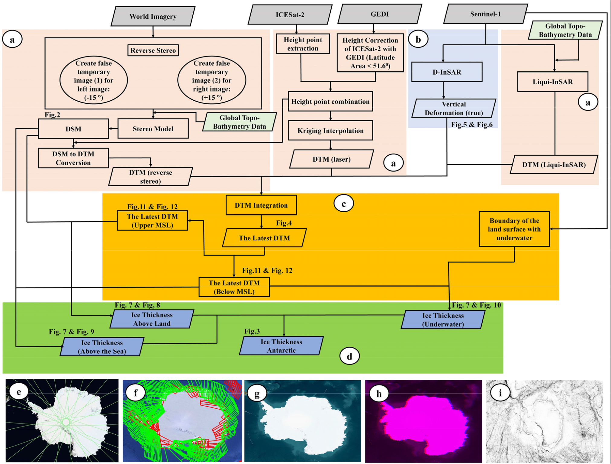
Fig. 1.

The workflow for measurement of Antarctica ice sheet thickness (above land, above the sea, and underwater). The measurement is based on the dynamics of land surface and underwater topography. There are four steps to measure the Antarctica ice sheet thickness: (a) DSM extraction of the surface layer of ice and topography with the latest DTM; (b) extraction of vertical deformation and the ice sheet thickness; (c) extraction of the latest DTM from the integration of DTM reverse stereo, DTM laser, DTM Liqui-InSAR with the latest vertical deformation; and (d) ice thickness of Antarctica calculation. (e) One of the trajectory of ICESat-2 data (2020); (f) The coverage of Sentinel-1 data (2021–2022); (g). World Imagery (2020); (h). Stereo model of World Imagery (2020); (i). Global Topo-bathymetry data

The three DTMs are used as input data in the next stage. These three types of DTM aim to ensure that all Antarctica regions complete their data with each other. DTM laser is extracted from the height points interpolation of raw data ICESat-2 and GEDI (2020). Height points are obtained from ICESat-2 and GEDI data. ICESAT-2 and GEDI data are used in the latitude region < 51.60, while in the latitude region > 51.60 only the ICESat-2 data is used. ICESat-2 data were corrected and correlated with height values from GEDI. This aims to increase the significance of DTM accuracy and precision, especially in latitude areas < 51.6° (Vernimmen et al. 2020). We can combine them due to GEDI has a narrower trajectory than ICESat-2. Next, height points are extracted for the latitude area < 51.60 and the latitude area > 51.60. All the height points data are combined, and Kriging interpolation is carried out. Kriging interpolation aims to model the DTM surface smoothly and minimize height errors. The Kriging interpolation input data is based on height points data from ICESat-2 and GEDI.

DTM Liqui-InSAR from underwater topography. Underwater topography was extracted using the Liqui-InSAR method (Julzarika et al. 2021a; Tarikhi 2012). Sentinel-1 data 2020 (SLC level) was used for underwater topography extraction. The extraction results obtained, namely underwater topography in 2020, are used as the DTM master (water) for the latest DTM extraction of water areas. The latest DTMs (land surface and underwater) are obtained by combining the two previously extracted DTMs. Based on these combined results, it can be seen that the area is above MSL and below MSL. This study also extracted underwater topography (2017) with Liqui-InSAR SAR images. It is used to determine the pattern of vertical deformation in the Antarctica waters. The Liqui-InSAR used the formula in equation (3) or equation (4) (Julzarika et al. 2021a).

where: 𝜆0 = the wavelength of SAR satellite 𝜃 = the incidence angle Q = co-factor matrix (1); e = random errors, calculate using least square adjustment. The value of surface currents is obtained from the earth and space research geoportal, and the value of surface winds prediction is calculated from Sentinel-1.

After obtaining the three types of DTM, the next step is to extract the latest vertical deformation. The latest vertical deformation extraction is the second stage of this research methodology. Vertical deformation is a model of deformation due to tectonic or volcanic movements, which shows the movement of the earth in a vertical direction up (uplift) and down (subsidence). It is characterized by geodynamics and influences topography and bathymetry dynamics. Vertical deformation monitoring can be carried out using direct measurements (terrestrial using Global Navigation Satellite System (GNSS)-Levelling/height difference measurements) and indirect measurements (satellites and aircraft using the InSAR/Differential InSAR (D-InSAR)/DTM difference method). The latest vertical deformation is the height difference of minimum two-period topography. We calculate it from D-InSAR or yearly vertical deformation velocity from Sentinel-1 (2020–2022). The vertical deformation (Line of Sight/LoS) has been corrected to be vertical deformation (true) using equation (5) (Suhadha and Julzarika 2022). The vertical deformation (true) is similar to the latest vertical deformation.

where 𝜃 = Sentinel-1 incidence angle

The 3^rd stage is the integration of all DTM with the latest vertical deformation; we call it the latest DTM. The latest DTM is obtained after integrating the DTM master on the latest vertical deformation. The DTM master in question combines the DTM reverse stereo, DTM laser, and DTM Liqui-InSAR. The extraction of the latest DTM is one of the methods and products to extract up-to-date and detailed topography based on the dynamics of the vertical deformation period. The latest DTM in this research is in December 2022. The DTM master 2020 is integrated with vertical deformation (January 2020–December 2022). The latest DTM can be extracted at any period. DTM before 2020 can also be extracted by integrating the vertical deformation according to the required period—for example, the DTM 2017 extraction. The method is to integrate the DTM master 2020 with vertical deformation (2020–2017). The integration process has considered the same height reference plane between the DTM masters with vertical deformation. We define the latest DTM in this research as integrating DTM reverse stereo, DTM laser, and DTM Liqui-InSAR with the latest vertical displacement. The latest DTM extracted is in the form of land surface and underwater topography. Equation (6) is used in the latest DTM extraction. It modified from the algorithm (Julzarika et al. 2021b) :

In the 4^th stage, we calculate the ice thickness of Antarctica. The calculation is based on the boundary of the land surface with underwater. The ice thickness calculation is divided into two parts: the calculation of the Antarctica land area and the Antarctica water area. The Antarctica land area uses the D-InSAR method with Sentinel-1 imagery (Caló et al. 2017; Devanthéry et al. 2016; Dias et al. 2018). The Antarctica waters area uses the results of the height difference of underwater topography (2020) and underwater topography (2017). Ice thickness extraction can be done using the ice sheet (DSM) and Antarctica topography (DTM) results. The ice thickness can be grouped into three, namely the thickness of the ice on land (ice thickness above land), the thickness of the ice with the upper surface above MSL but the lower surface below MSL (ice thickness above the sea), and the thickness of the ice below MSL (ice thickness in underwater).

Ice sheet thickness calculation using the volume formula with the cut-and-fill method (Baek and Choi 2017; Kubla 2019). The method uses the bottom of the layer (elevation in land surface and underwater topography) as a zero-reference plane for volume calculations. The cut-and-fill method is a soil or ice surface work process in whic h several materials, soil, ice surface, or rocks, are taken from a particular place and then moved to another place to create the desired elevation. The cut-and-fill method makes it easy to calculate the volume because the elevation and height differences are known based on the zero-reference plane.

The volume calculation based on cut-and-fill uses the grid method (Kubla 2019). The grid method describes a uniform grid on each soil surface that is cut and filled. Each grid will have an elevation value and a different elevation according to the cut and fill sections (Julzarika 2015). The volume of each pixel is obtained by multiplying the depth by the pixel area or the project area. The total cut and fill volume is obtained by adding each pixel together (Kubla 2019).

3. Results and Discussion

The main result of this research is information about measuring the thickness of the Antarctica ice sheet. The ice thickness is divided into three: ice thickness above land (based on the DTM 2022), ice thickness above the sea (based on the DSM 2022), and ice thickness underwater (based on bathymetry). To obtain the main results of this research, supporting research results are needed, including DSM and DTM Antarctica 2022, bathymetry, and vertical deformation. The vertical accuracy of the DTM, DSM, and vertical deformation uses a 95 % (1.96σ) confidence level.

The DSM Antarctica 2022

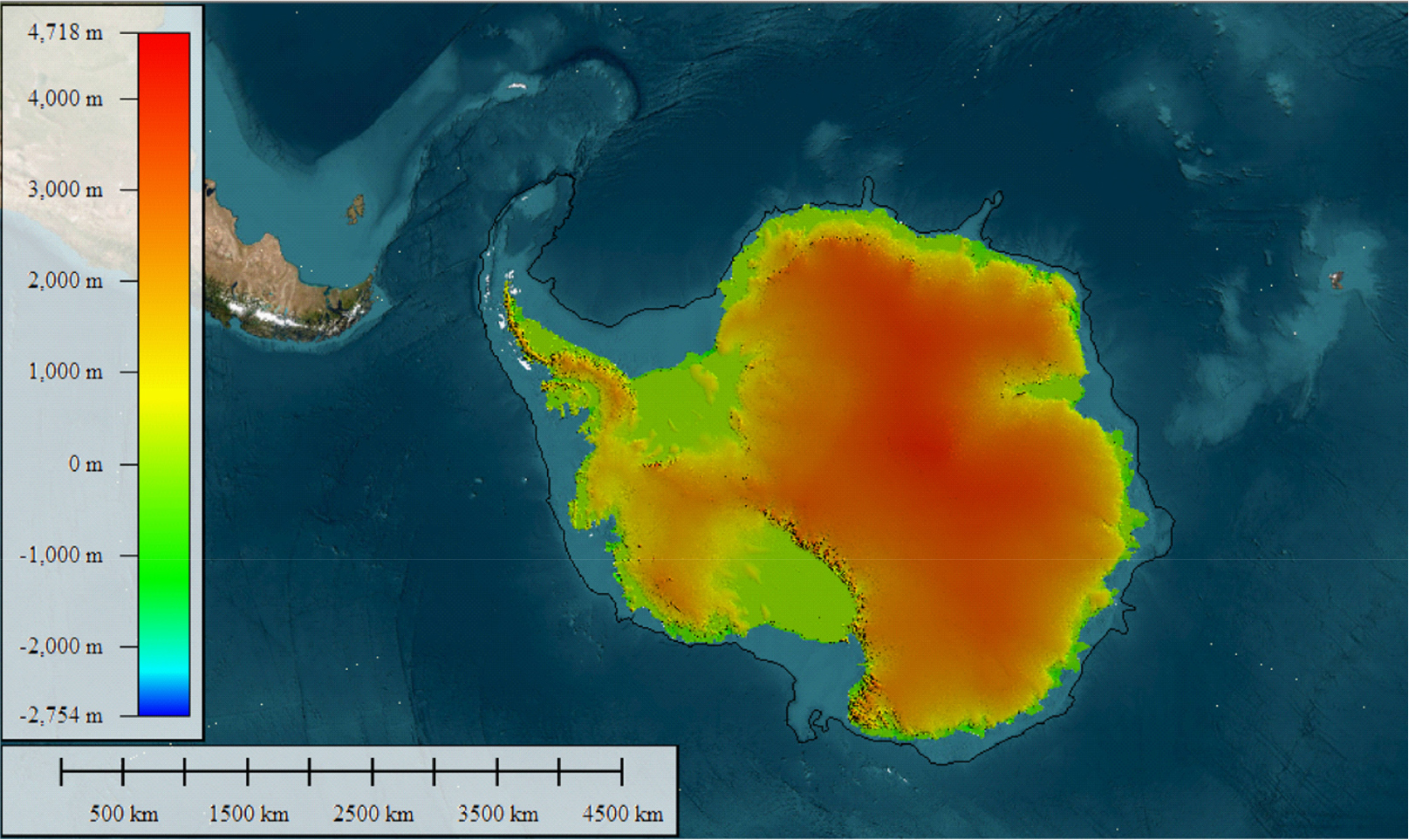
The extracted DSM Antarctica displays the ice surface layer only above the water. The DSM Antarctica extracted from a combination of World Imagery, ICESat-2/GEDI, and Sentinel-1 data have various elevations. The updated DSM 2022 uses ICESat-2/GEDI and Sentinel-1 data. DSM 2020 extracted from World Imagery data. The elevation still describes the ice sheet surface.

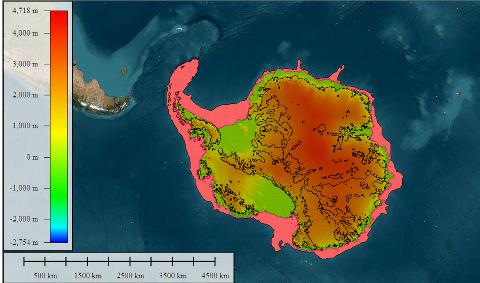
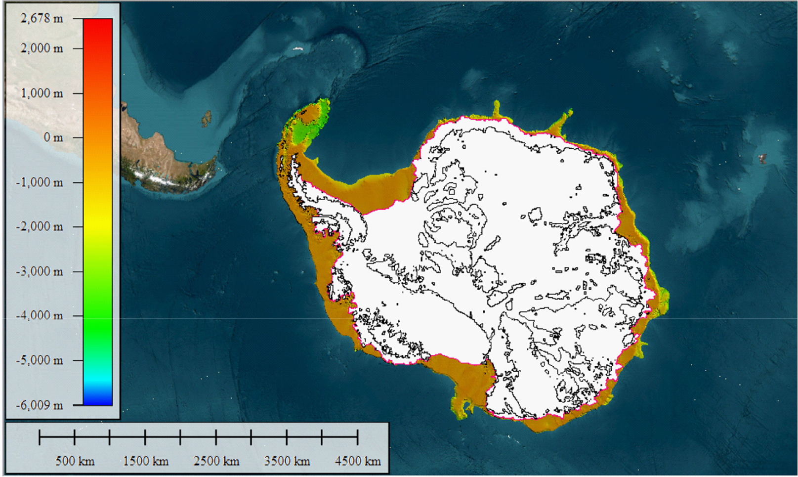
The DSM Antarctica 2022 display can be seen in Fig. 2. The elevation value is at -2754 m to 4718 m. The elevation value does not describe the coastline condition and topography height. To determine land surface topography, underwater topography, and ice thickness, a DSM to DTM conversion is required. The DSM Antarctica elevation is at a value of 1000 to 4718 m. The elevation on the west and part of the north coast is < 1000 m. Some areas to the west also have elevations below MSL (< 0 m). The areas with the highest elevations are in the landmass’s central part, extending from north to southeast Antarctica. The black line in Fig. 2 represents the potential for ice sheets in Antarctica, both those still on the land surface and those that have melted and left an ice layer under MSL.

Fig. 2.

The DSM Antarctica 2022

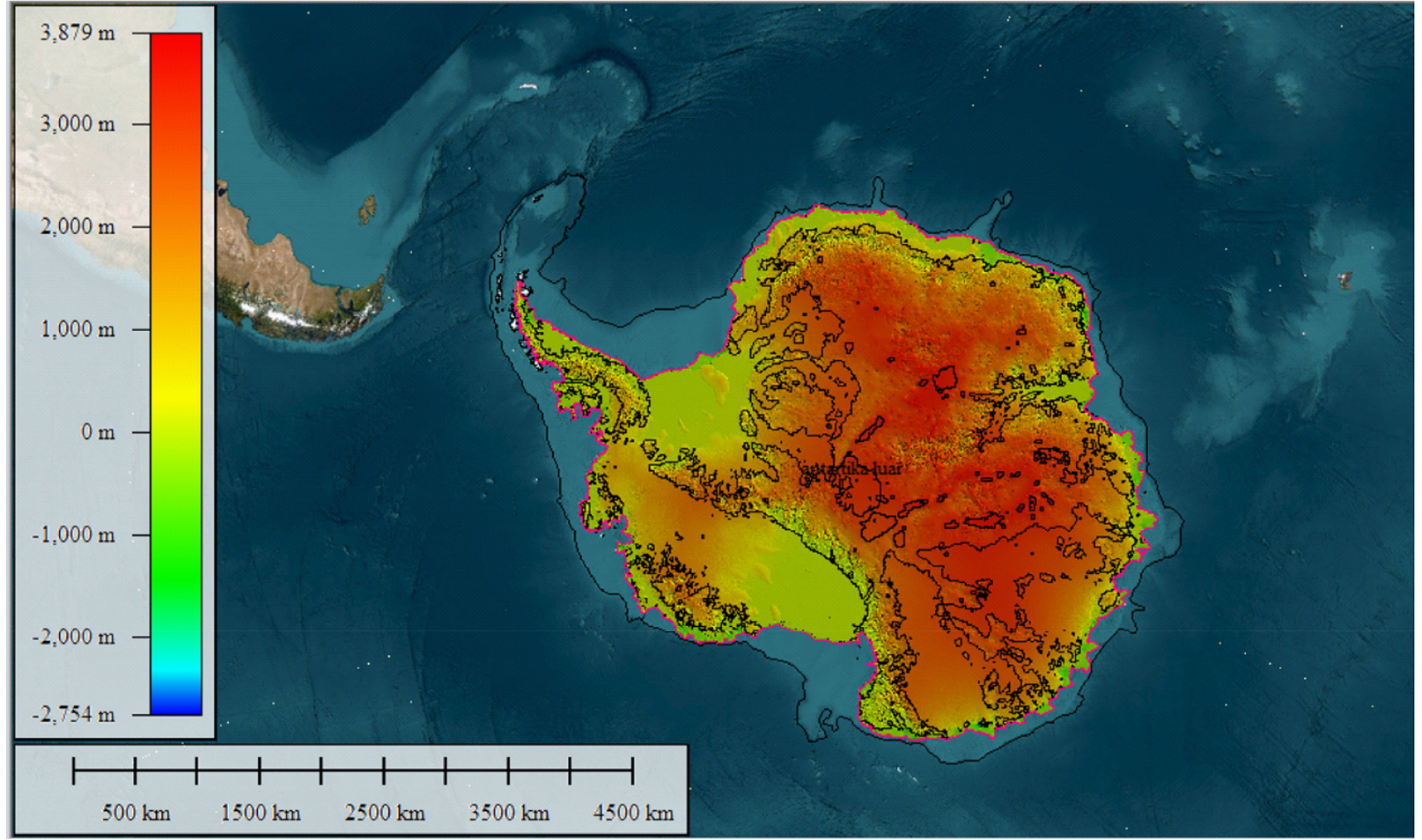
The areas with black lines in Fig. 3 represent the potential of the entire Antarctica ice sheet. The remaining ice layer can be identified using the latest DTM (underwater topography). The potential of all ice potential in Antarctica is extracted by using the integration of DSM with underwater topography. Fig. 3 shows the potential of all ice sheets in Antarctica in 2022.

Fig. 3.

The potential of all ice sheets in Antarctica 2022

The DTM Antarctica 2022

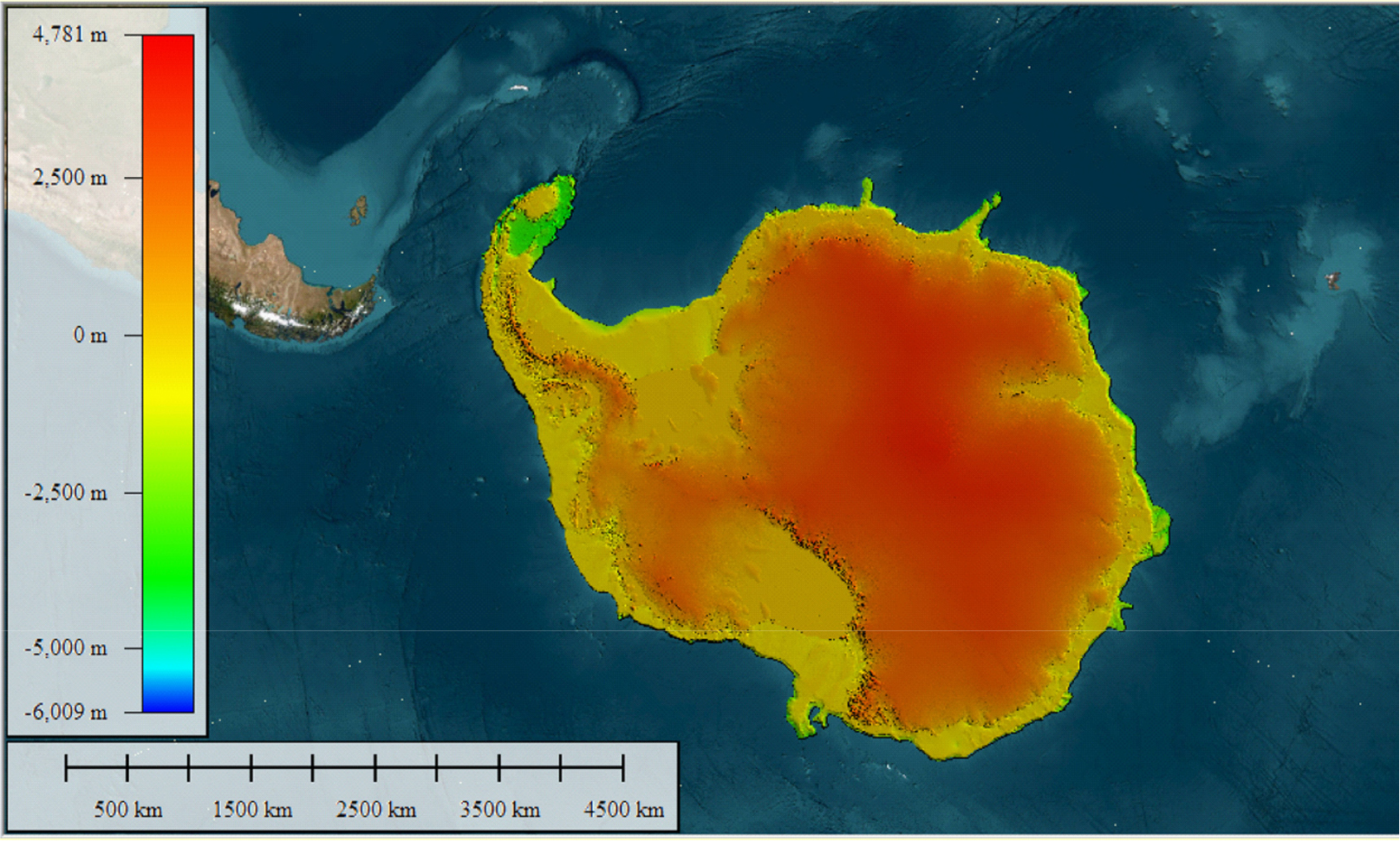
The DTM Antarctica 2022 results from reducing the DSM Antarctica with the potential ice thickness and it is bedrock topography. The latest DTM for the Antarctica region in 2022 is extracted from the results of DTM Antarctica with the vertical deformation (2022) integration. The horizontal datum used in the latest DTM Antarctica is the Polar Stereographic. Based on the latest DTM Antarctica 2022 results, DTM boundary lines are extracted, which can be used to calculate the area and volume of Antarctica in 2022.

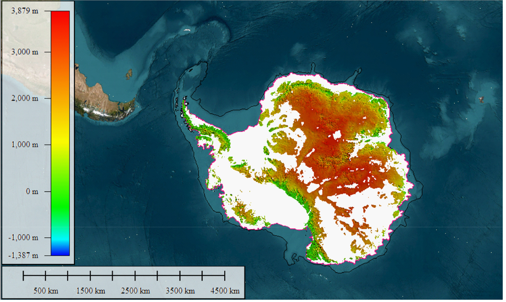
Based on the latest DTM conditions for 2022, it can be seen that Antarctica is more dominated by ice sheets that lie under MSL (underwater topography). Ice sheets in topography areas (land) are less than 40% of the total ice sheet (mainland of Antarctica). Fig. 4 is the latest DTM Antarctica 2022. The DTM integration results from the DTM master (land), DTM master (water), and vertical deformation. The pink area in Fig. 4 is the predicted ice sheet area already under MSL. It is no longer connected with the ice sheet above the topography. The area that is colored cyan is the ice surface layer with the condition that the top surface is above MSL and the bottom is below MSL. The cyan-colored area is included in the underwater topography category. The ice layer is still continuous, with the ice layer above the land surface topography. The area in blue-green-yellow-orange-brown is the land surface topography in Antarctica. This area is the land located under the ice thick layer.

Fig. 4.

The DTM Antarctica 2022

The vertical deformation of Antarctica

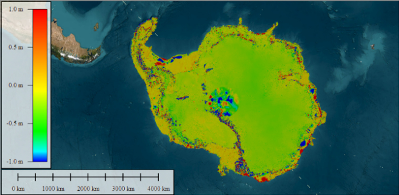
The vertical deformation in Antarctica during the 2014–2022 was -5 m to 2 m. Some areas where ice avalanches occurred are marked in cyan and blue in Fig. 5. Ice slides generally occur on the coast of the Antarctica ice sheet. It also occurs along the Transantarctica Mountains. Uplift in the ice sheet also occurs in the Antarctica region. The area is in a location adjacent to the ice slide. In addition, the ice addition also occurs on the coast, which is affected by the dynamics of seasons, currents, and sea waves. The uplift of the ice layer is marked in orange-red. Fig. 5 shows the vertical deformation in Antarctica and the surrounding waters in 2014–2022. This vertical deformation is used to update the results of DSM, DTM, and bathymetry extraction. Vertical deformations were extracted in Antarctica and the surrounding waters in 2014–2022.

Fig. 5.

The vertical deformation in Antarctica and the surrounding waters in the period 2014–2022

The average speed of vertical deformation in the Antarctica region is relatively high, which is -50 cm to 10 cm per year. The Antarctica region is dominated by subsidence, while the waters around the Antarctica region are dominated by uplift. The overall rise of the ocean floor can cause changes in the dynamics of undercurrents and surface currents. Uplift in the Antarctica waters is affected by active tectonic/seismic movements, marked by the many occurrences of large earthquakes. Antarctica waters include the Atlantic, Hindia, and Pacific Oceans. The effect of this uplift is more dominant on changes in the Antarctica environment. In contrast, the effects of sea level rise and the environment do not significantly affect vertical deformation. Fig. 6 is the average velocity per year of vertical deformation in Antarctica. The average vertical deformation velocity per year can also be used to determine Antarctica’s tectonic dynamics, ice melting, and the addition of ice sheets.

Fig. 6.

The average velocity per year of vertical deformation in Antarctica

The distribution of ice sheet and ice thickness of Antarctica 2022

The DSM Antarctica 2022 is used to determine the distribution of ice sheets based on the ice thickness. The ice sheet distribution is divided into three, namely the ice thickness below sea level or located underwater (pink color), the ice thickness with the peak above sea level, and the base below MSL or located above the sea (areas other than pink and black line), and the ice thickness above MSL or located above land (black line). Fig. 7 is the ice sheet distribution based on the ice thickness.

Based on the ice sheet distribution in Fig. 7, we classified the ice thickness into three categories: ice thickness above land, ice thickness (above the sea), and ice thickness (underwater). All of this ice thickness is in the period 2022.

Fig. 7.

The distribution of ice sheets is based on the thickness of the ice

Ice thickness above land in 2022

The thickness of the ice on the mainland is obtained from the results of the height difference between the DSM (surface layer) and the DTM (land surface topography). The thickness of the ice has a volume of 3,700,299,528,458,631 m³ (3,700,299.5 km³) with an area of 6,767,772 km². The total length perimeter of this area is 114,569 km. Fig. 8 is a display of the ice thickness of the Antarctica continent. This Antarctica land surface topography area has a thick layer of ice, and there is still little possibility of shrinkage. One of the causes of ice shrinkage in this category (1) region is the high vertical deformation anomaly.

Fig. 8.

The ice thickness of Antarctica

Ice thickness (above the sea) in 2022

The ice thickness above the sea means that the surface of the upper layer is above MSL or continuous with the ice sheet above the land, while the lower layer is below MSL or in underwater topography. The ice thickness of this category has a volume of 28,103,427,808,066,548 m³ (28,103,427.8 km³) with an area of 13,438,789 km². The total length perimeter is 27,199 km. Fig. 9 displays Antarctica’s ice thickness (above sea) in 2022. This category (2) area is still vulnerable to ice shrinking, especially in its coastal areas (purple line). These vulnerable areas are affected by seasonal conditions, currents, sea waves, vertical deformation, and seismic/tectonic movements. The area can experience ice shrinkage, which can also occur with adding ice cover. The white areas (between the purple and black lines) of Fig. 9 still have a thick layer, and there is little chance of shrinkage. The high vertical deformation anomaly in this category (2) area can cause rapid and sudden ice shrinkage.

Fig. 9.

The ice thickness (above sea) of Antarctica

Ice thickness underwater in 2022

The ice thickness (underwater) is located under MSL and is already under the sea. The ice thickness in this category has a volume of 1,793,778,616,625,720 m³ (1,793,778.6 km³) with an area of 3,223,036 km². The total length perimeter of this area is 46,556 km. This area was previously ice thickness category (2), but due to the ice shrinkage, there is currently a lot of ice melting. The high vertical deformation anomaly in the category (3) region can cause rapid ice melting. Fig. 10 is the ice thickness (underwater) of Antarctica.

Fig. 10.

The ice thickness (underwater) of Antarctica

Profile test of the ice thickness

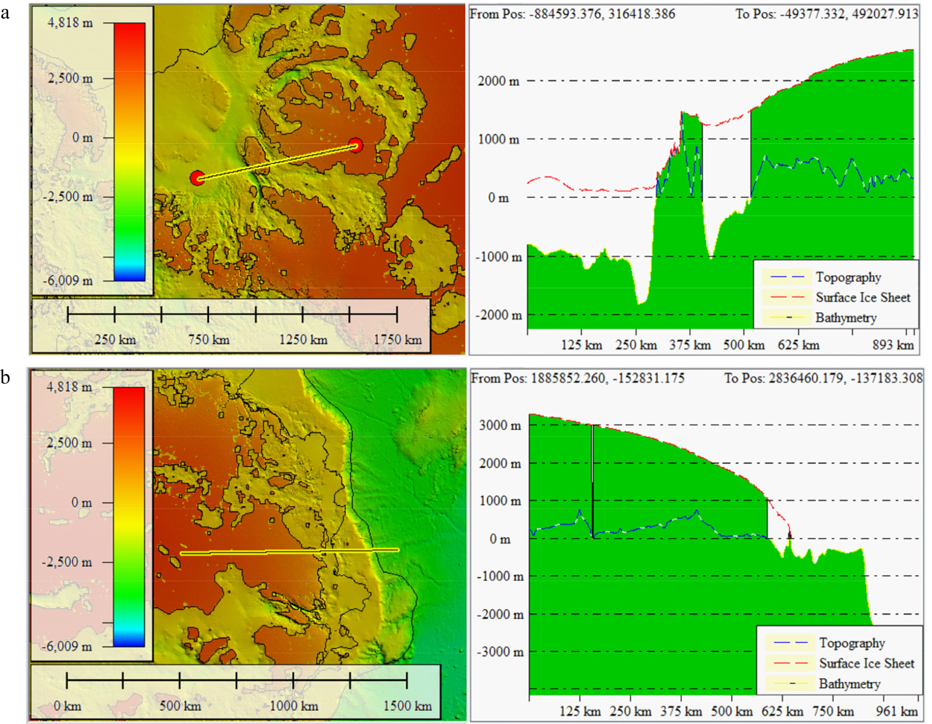
Profile test is used to check the quality of the appearance of the ice surface, land surface topography, and underwater topography. Two types of profiles are used in geo-modelling, namely the cross-section profile and the longitudinal profile. The cross-section profile to view the ice sheet and Antarctica topography. It is used to check the shape of the ice thickness display. A cross-section profile is made to cut the Antarctica area from west to east or from underwater topography to the mountains.

Fig. 11a is a cross-section profile in the West Antarctica region, while Fig. 11b is a cross-section profile in the East Antarctica region. The blue line is a topography display of the land. The red line shows the surface of the ice layer. The yellow line is a bathymetry display. From these two figures, we can see the two types of ice thickness. Two types of thickness can be seen: the ice thickness above the Antarctica continent (the area between the red line and the blue line) and the ice thickness calculated from the surface of the underwater topography (bathymetry).

Fig. 11.

The cross-section profile of Antarctica. In the legend, the topography is similar to land surface topography; bathymetry is similar to underwater topography. (a). location in West Antarctica. (b). location in East Antarctica

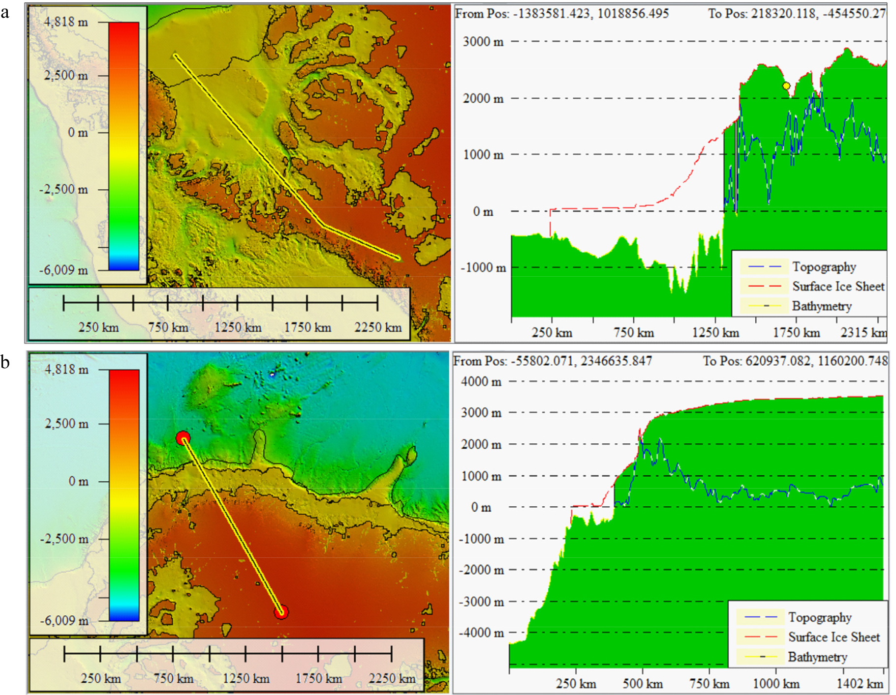
The longitudinal profile is used to view the ice sheet and Antarctica topography and to visualize the ice thickness from north to south or in the direction of the Transantarctica Mountains. On checking with this longitudinal profile, the ice thickness is thinner as it passes through the mountains. Antarctica's coastal areas have thinning ice as well. Visually, the thickness of the ice on land can be seen in Fig. 12a, located between the red line (ice sheet surface) and the blue line (land surface topography).

The ice thickness calculated from underwater topography is located between the red and yellow lines (underwater topography). In Fig. 12b, it can be seen that the ice layer has melted. The absence of a red line above the yellow line indicates this. An example of the loss of ice sheets can also be seen in Fig. 12a; on the left side of the longitudinal profile graph, there is no red line above the yellow line.

Fig. 12.

The longitudinal profile of Antarctica. In the legend, the topography is similar to land surface topography; bathymetry is similar to underwater topography. (a). location in West Antarctica. (b). location in East Antarctica

The results of this study need to be compared relatively with other similar studies because it is not possible for field checks in Antarctica. Several other studies have calculated the ice thickness of Antarctica such as (Bamber and Griggs 2009; Dorschel et al. 2022; Lemenkova 2021; Paxman et al. 2019; Znachko-Yavorskiy 1978). Paxman et al. 2019 researched the reconstructions of Antarctica's topography since the Eocene-Oligocene boundary. A realistic reconstruction of bedrock evolution is necessary to obtain an accurate model of the Antarctica ice sheet. The study was conducted at the Eocene-Oligocene boundary with four central time slices in the Antarctica climate, namely the Eocene-Oligocene boundary (ca. 34 Ma), the Oligocene-Miocene boundary (ca. 23 Ma), the mid-Miocene climate transition (ca. 14 Ma), and the warm period of the mid-Pliocene (ca. 3.5 Ma). The process of ice sheet loading, isostatic adjustment flexure, sedimentation, horizontal plate movement, thermal subsidence, volcanism, erosion, and onshore and offshore geological boundaries was considered in past reconstructions. The results of this study suggest that the current land area of Antarctica, which is located above sea level, is ~25% larger at the Eocene-Oligocene boundary Antarctica ice sheet and it has implications for estimating changes in global ice volume, temperature, and sea level across major Cenozoic climate transitions. The layer 0 to 500 m above sea level is particularly vulnerable to ice sheet retreat. The catchment-averaged erosion rates are on the order of 10–20 m/Myr. The latest DTM Antarctica research also found conditions in several locations with elevations of 0 to 500 m, which are vulnerable to ice melting and causing a decline in the surface line of the ice sheet.

Znachko-Yavorskiy 1978 researched the topography of Antarctica. The research mapped subglacial bedrock topography and Antarctica ice thickness. The East Antarctica region experiences a dominant uplift of subglacial relief. These conditions lead to a greater ice thickness. The ice thickness is more than 3000 m. West Antarctica is experiencing predominant bedrock subsidence. These conditions cause the ice thickness not to exceed 3000 m. In the latest DTM Antarctica research, the thickness of the ice obtained is generally more than 3000 m or in the range of 3000 to 4000 m. This ice thickness occurs in the East Antarctica region. In the West Antarctica region, the ice thickness ranges from 1500 to 2500 m or generally less than 3000 m. Other parts of this region have ice thicknesses of 0 to 1500 m. If the relative accuracy test is carried out between the ice thickness research and the latest DTM with ice thickness Znachko-Yavorskiy 1978, the relative vertical accuracy value is still in the 1.96 σ (95%) range. The comparison uses the thickness of the West Antarctica and East Antarctica ice based on the difference between the research results.

Bamber and Griggs 2009 researched the creation of a 1 km DEM Antarctica with a combination of the ERS-1 radar and the ICESat laser altimetry satellite. The accuracy of the DEM uses an independent airborne altimeter data set, and it is used to generate a height error map. In the latest DTM Antarctica study, the results can also be used to estimate ice thickness, land surface topography, underwater topography, vertical deformation rate, and Antarctica land dynamics (ice surface melting rate). Lemenkova 2021 researched compiling datasets with GRASS GIS for Antarctica thematic mapping. This research determines land surface topography, ice thickness, sediment thickness, and subglacial bed elevation. This study uses the results of data compilation ETOPO1, GlobSed, EGM96, and Bedmap2. Geospatial processing algorithms modify all data compilations. Then, geo-visualization is carried out on the processed DEM results. The results of the geo-visualization can be used to determine ice surface topography and the bedrock elevation, ETOPO1-based surface and underwater topography, geoid undulation, and ice sheet thickness. The latest DTM Antarctica research can also be used to determine the topography and bathymetry elevation and predict the ice sheet thickness.

Dorschel et al. 2022 researched making a new version of the international bathymetry map (southern polar circle). Since 2013, the underwater topography of the Southern Ocean south has been represented by the International Bathymetry Chart of the Southern Ocean (IBCSO). The IBCSO Project has collaborated with the Nippon Foundation -GEBCO Seabed Project 2030 to support the global ocean mapping goal 2030 (IBCSO v2). Its territory covers up to 50° S (2.4 times the seafloor area of the previous version), including the Antarctica Arctic Circle Current gateway and the Antarctica circumpolar frontal system. IBCSO v2 will significantly increase the representation of the Southern Ocean’s seafloor and resolve underwater landforms in greater detail. This condition was caused by the increased data coverage (multi-beam). The latest DTM Antarctica research also produces land surface topography and underwater topography. The geo-forensics approach can reconstruct the previous land surface and underwater topography conditions. The difference between the land surface and underwater topography (height difference) in the previous period will produce information on the vertical deformation rate. The vertical deformation covers the Antarctica waters and land areas (bedrock).

4. Conclusions

The Antarctica ice sheet thickness can be detected and calculated based on land surface dynamics and underwater topography extracted from the latest DTM. Three types of ice thickness can be calculated, namely ice thickness above land, ice thickness (above the sea), and ice thickness (underwater). Ice thickness above land has a volume of 3,700,299.5 km³ with an area of 6,767,772 km². The total length perimeter of this area is 114,569 km. The thickness of the ice above land is calculated based on the height difference between the surface of the ice sheet (DSM) and the topography (DTM). Ice thickness (above the sea) has a volume of 28,103,427.8 km³ with an area of 13,438,789 km². The total length perimeter is 27,199 km. The ice sheet’s thickness (above the sea) is calculated based on the difference in height of the surface layer of ice (DSM) with underwater topography. Ice thickness (underwater) has a volume of 1,793,778.6 km³ with an area of 3,223,036 km². The total length perimeter of this area is 46,556 km. The ice sheet thickness is below MSL and under the sea. The period and the ice sheet thickness are adjusted to the vertical deformation time used in the latest DTM extraction. The average vertical deformation velocity per year can also be used to determine Antarctica’s tectonic dynamics, ice melting, and the addition of ice sheets. The vertical accuracy of the DTM, DSM, and vertical deformation uses a 95 % (1.96σ) confidence level.