

1. Introduction
2. Materials and Methods
Materials
Missing of chlorophyll to sea grids ratio
Spatial autocorrelation index of missing-grids locations
Pattern analysis of spatial point distribution
Seasonality analysis
3. Results and Discussion
Variation of missing ratio (MR) for different integrating periods
Variation of Moran’s I for different integrating periods
Variation of K-function for different integrating periods
Seasonality of MR
4. Summary & Conclusions
1. Introduction
Satellite image has been one of the outstanding source for marine monitoring and surveillance due to its extensive and regular observation in spatial and temporal aspects more than traditional methods using cruising ships, stationary buoys and stations.
However, optical satellite-based marine observations have significant challenges, data transformation, and missing. First, data transformation depends on developing algorithms to estimate the values of their aimed variables. On the other hand, data missing caused by high aerosol ratio, cloud, and others is a more critical barrier to utilizing optical satellite images. Accordingly, the availability of satellite images depends on its missing ratio and missing pattern.
Most research on utilizing optical satellite images has been focused on developing algorithms to convert satellite- observed radiance into desired variables or on assessing satellite-based products. However, data missing has been a decisive obstacle to the use of satellite-based products (Mercury et al. 2012; Robinson et al. 2019; Stock et al. 2020). Hence, the use of satellite-based products requires spatial-statistics analysis in advance. Mercury et al. (2012) compared cloud geographic features for the exact date of single day image and consecutive 5 and 10 years-composite images for landmass. The more compositing years, the more obvious graphical features apparent. Robinson et al. (2019) investigated cloud cover during earthquakes seasons on a global scale. They then insisted on avoiding dependency on optical satellite images because 40% of the global population is in danger when a cloud covers optical satellite views. Stock et al. (2020) compared spatial interpolation methods such as IDW (inverse distance weight), kriging, DINEOF (data-interpolating empirical orthogonal functions), and machine learning such as ridge regression and random forest. Then he/she found spatial interpolation is preferable in gap-filling approaches rather than machine learning methods.
The research described above focused on data conversion and filling, not how the missing grids have distributed on temporal and spatial axis. Thus, this report aims to quantitatively evaluate the spatial distribution of missing and give insight into the use of optical satellite images and products. First, we review flags, marked as the reason of missing data, in Geo Stationary Ocean Color Imager I (GOCI-I) chlorophyll concentration product, estimate and analyze the three-years temporal trend of missing ratio by the temporal and spatial integration scale. Then we estimate spatial autocorrelation coefficients and spatial randomness from the distribution of missing grids.
2. Materials and Methods
Materials
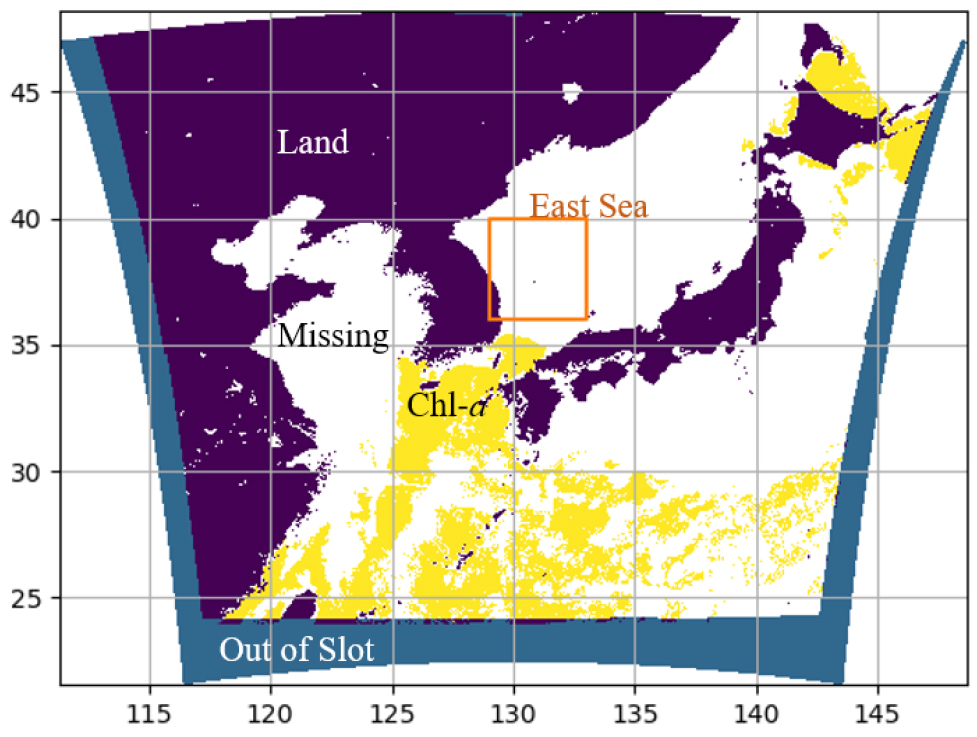
GOCI-I is one of the payloads on Communication, Ocean, and Meteorological Satellite (COMS). GOCI-I carried out its mission to monitor the atmosphere and ocean from June 27, 2010, to March 31, 2021, and GOCI- II on satellite GEO-KOMPSAT-2B has succeeded the duty. The GOCI-I image covers East Asia with approximately 2,500 km2, centered on Korea, consisting of 5,585 by 5,567 pixels in the vertical and horizontal axis, with orthogonal projection. Research areas are divided into two to compare the regional characteristics of the missing ratio. One is overall GOCI-I coverage explained above, and another is East sea of Korea, ranging approximately from 129° to 133° in longitude, from 36° to 40° in latitude (Fig. 1).
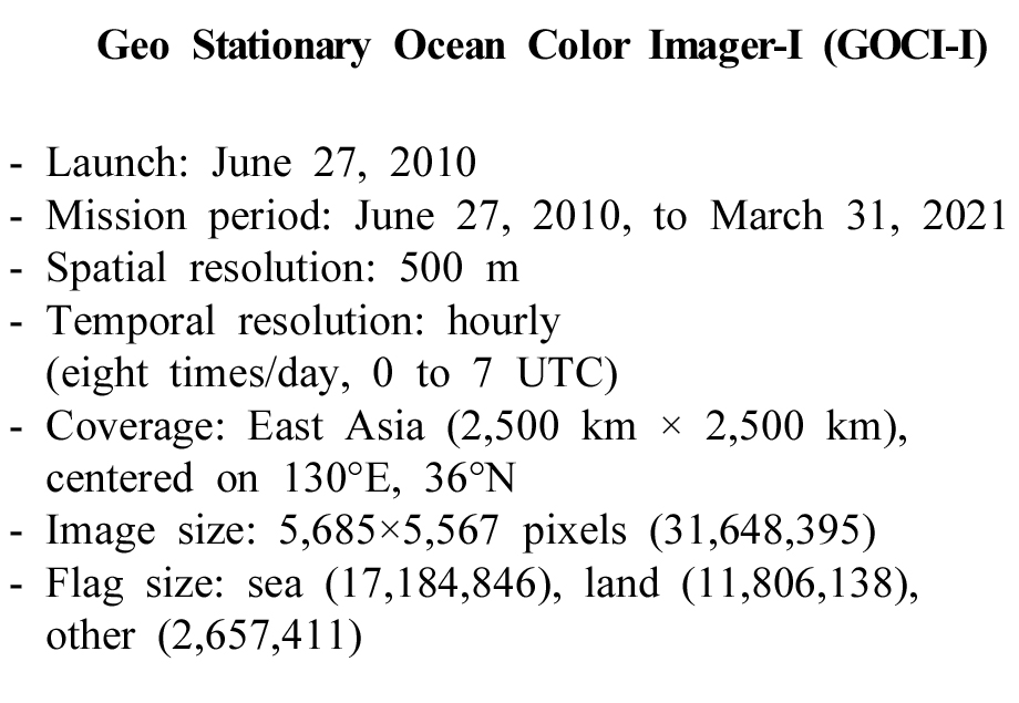
In general, eight GOCI-I images are produced per day with hourly intervals from 00:15 to 07:45 UTC, and their spatial resolution is 500 m. In addition, GOCI-I has eight optical bands from between 400 to 900 nm, including NIR (near-infrared); after that, it has contributed to observing chlorophyll, turbidity, and suspended matter in the sea as well as the atmosphere (Kim et al. 2016; Jeon et al. 2020).
The data we used in this report is chlorophyll concentration product at level2a (L2A) estimated from GOCI-I. The period is from March 04, 2018 to March 26, 2021 (approximately three years, total of 1,119 days). Although it has a difference in the number of observations per day due to seasonality, it generally has eight observations per day (Table 1). There are eight days of non-observation, May 8 to 13, 2019(6 days) and June 22, 2019, to January 26, 2020, among the period. Consequently, 1,111 days, subtracting eight days from 1,119 days, were used in this report.
Table 1.
GOCI-1 image data used in this note
Items No. of images/Day | Days | No. of images | Season* |
| 3 | 1 | 3 | summer |
| 7 | 31 | 217 | winter |
| 8(normal) | 1,059 | 8,472 | - |
| 9 | 10 | 90 | - |
| 10 | 4 | 40 | summer |
| 11 | 3 | 33 | summer |
| 12 | 1 | 12 | summer |
| 16 | 2 | 32 | spring |
| Total | 1,111 | 8,899 |
The chlorophyll products are available at Korea Ocean Satellite Center (KOSC) website (http://kosc.kiost.ac.kr), operated by Korea Institute of Ocean Science and Technology (KIOST). The chlorophyll products are formatted in HE5, hierarchical data format release 5, which can contain chlorophyll concentration and flag, map projection, radiometric calibration, and others. Its size is approximately 120 MB per image.
GOCI-I defines 28 flags to minimize the error of the estimated the values of products. The specific flag for missed chlorophyll data is summarized using the rayleigh corrected reflectance products at level2c (L2C) and the chlorophyll products at L2A (Table 2). Ten samples were chosen considering minimizing the effect of seasonality and illumination of sunlight, 2018-Apr-20 06:16, 2018- Aug-06 00:16, 2018-Sep-10 07:16, 2018-Dec-14 00:16, 2019-Jun-23 03:16, 2019-Jul-03 03:16, 2020-Feb-24 06:16, 2020-Apr-29 05:16, 2020-Jul-13 03:16 and 2020-Aug-20 03:16.
Table 2.
Flags effect on missing of chlorophyll concentration
Flag to Chlorophyll Missing Ratio (FCMR) uses the number of chlorophyll missing pixels on the overall area as the denominator. In contrast, Flag to Chlorophyll Missing at Sea Ratio (FCMSR) uses the number of missing grids at sea as the denominator, determined after subtracting “Land” and “OUT_OF_SLOT” flags from overall grids. In addition, the values on ‘10 samples’ indicate the median of them, whereas ‘Apr. 20, 2018’ indicates the first sample, 2018-Apr-20 06:16.
Flags are obtained from GOCI-I Rayleigh corrected reflectance products because chlorophyll products do not contain flags themselves. Among the top ten flags, “Ancillary_Data_Warning” indicates an anomaly determined through five-years average trend. “Cotm_Pxl_Warn” is the contaminated pixel from more than two flags. “High_ Aerosol_Ratio” is the pixel having aerosol reflectance over three-times water reflectance at any band. “Rrs_ Spectrum_Shape_Wrong” is the pixel having unrealistic remote sensing reflectance (Rrs). “Negative_Lw” is the case where water-leaving radiance is less than zero. “Cloud_ or_Ice” is the case where exceeds 0.03. “Negative_RhoC_NIR” is the pixel that rayleigh corrected radiance is less than zero. Finally, “Atmospheric_ Correction_Fail” is the case where is not retrieved from . and represents multiply scattered aerosol reflectance and reflectance of interactively scattered between aerosol and molecular. and represents the band of visible and near- infrared.
Missing of chlorophyll to sea grids ratio
The missing chlorophyll data to sea grids Ratio (MR) is computed after extracting sea area by subtracting “Land” and “OUT_OF_SLOT.” MR is a reference to understand the proportion of the missed chlorophyll concentration data at sea in the image. The missing grids occur for various reasons, as referred to in section 2.1. MR is computed for every hourly image. All the sea grids with chlorophyll concentration are converted into integer one (1) instead of the actual value, and the grids without data are converted into value NaN (-). Thus, we have binary information to determine the grids’ observation status between presence (1) and absence (0). The Daily Mode (DM) is generated to reduce the number of missing grids (Fig. 2a).
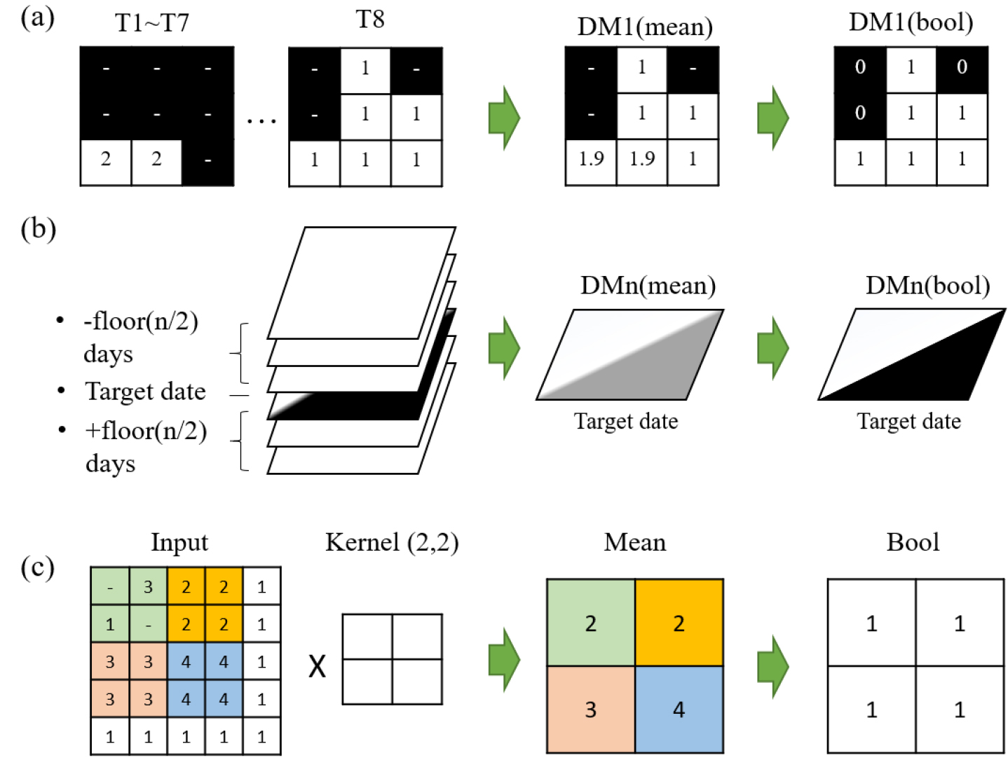
DM is generated through the temporal integration process. First, hourly images on a day are accumulated on a time axis. Then the individual spatial grid is examined whether it has any missing on the time axis. If there is missing, the grid has integer zero (0), unless otherwise, the grid has integer one (1). Consequently, the increasing number of integration images causes a decrease in missing grids. Then DMn - represents the days of integration - is made for 3, 5, 7, and 9 days each by using the DM (Fig. 2b). Then the DM and DMn are formatted in NetCDF, array-oriented scientific data, having file extension NC.
The DMn indicates whether it has at least one piece of information for a given grid over a specific period. Like temporal integration bring a missing reduction effect, spatial integration also brings a missing reduction. Thus, square matrix kernel is used, increasing the value of , to compare the effect of missing reduction upon the kernel size (Fig. 2c).
Spatial autocorrelation index of missing-grids locations
Before computing spatial autocorrelation of GOCI-I missing grids, DMn is scaled into 100 by 100 pixels, since the original size, 5,585 by 5,567 pixels in the vertical and horizontal axis, leads to too massive computation works.
Both overall coverage and the East sea of the GOCI-I are analyzed through Moran’s I, one of the representative spatial autocorrelation indices, to evaluate how the missing grids correlated one to neighbors (Cliff and Ord 1969; Anselin 1995; Jossart et al. 2020). The weights required to compute the respective index are calculated using IDW (inverse distance weight), the inverse of the distance between missing grids (Eq. 1).
Moran’s I is computed through Eq. 2.
where, denotes the number of all grids corresponding to ocean, denotes the summation of all weights (), (,) denotes whether missing grids is true (1) or false (0). denotes arithmetic mean of every grids expressed 1 or 0, and : weight computed by the function of distance between two grids (,).
Pattern analysis of spatial point distribution
Pattern analysis of spatial point distribution begins with the null hypothesis of complete spatial randomness (CSR), in which spatial grids are homogeneous and isotropic in space. Hence, test whether the distribution of data matches CSR.
To evaluate the randomness or cluster of cloud cover, K-function, one of the distance-based spatial point pattern functions using R package “spatstat”(Baddeley and Turner 2005). K value is computed using Eq. 3. The nominator denotes that the number of events where two points () distance is less than specific distance while the denominator represents that ratio of the number of every combination of two points in the unit region to the area of unit region ().
where, denotes the number of events where two points distance is less than , denotes the distance between points and (≠), and denotes the ratio of to the area of the unit region ().
On the other hand, the K value that represents CSR can be expressed as in Eq. 4. Once the distribution of spatial points is independent, that is not affected by the other, and the random variable of the distance between two points () can be assumed as the spatial randomness and independent. Thus Poisson distribution can be considered here. Given that the density of points () and the variable of distance are constant, the number of combinations within a specific distance is proportional to the circle are with radius r().
If is higher than ,
Seasonality analysis
Although we might assume a seasonality in time-series graphs by glancing, reasonable seasonal periods can be computed from Fisher G-test and Whittle test (Fisher 1929; Hernandez 1999; Akmaev 2003; Cho 2020). The basic is the harmonic analysis that finds trends and periods in time-series data. Specifically, harmonic functions such as sine and cosine are widely used for spectrum analysis, Fourier transform and fast Fourier transform (FFT) related to the frequency that is inversed period.
The periodogram method is chosen to analyze frequency which will be converted into a period. The periodogram is a diagram that illustrates the magnitude of the coefficient of Fourier transform and is thus useful to detect superior frequency. The magnitude was computed using R package “TSA”. Given that the magnitude of frequency is significant, the frequency is adopted as a reasonable one, and then the inversed value of frequency becomes the principal period. F-value and F-critical value were first computed using Eq. 5 and R function “qf” to obtain significant frequency candidates through threshold value (Weerahandi 1995).
where, denotes the number of data, denotes the magnitude of Fourier transform coefficient, denotes angular frequency.
The statistics for the periodicity test are computed using Eq. 6 & 7. Fisher statistics is used to get for the primary magnitude of frequency while Whitle statistics is used to get from the second magnitude of frequency.
where, subscript denotes rank of the in descending order.
In fact, the exact critical value is computed through a complicated equation in accordance with Fisher test method and thus we use the approximate formula, in which the significant level (α) is 0.05(Eq. 8) Given that is greater than , it means the frequency is significant to stand for periodicity in -th order. Inversely, the contrast case means the null hypothesis of none seasonality is adopted.
where,
3. Results and Discussion
Variation of missing ratio (MR) for different integrating periods
The temporal integration was made from March 4, 2018, to March 26, 2021, through the method described in Fig. 2 above. Hourly image (HR1) shows the highest MR with an average of 80.6%(Fig. 3). Thus HR1 is not proper data to monitor the wide sea area. DM3 shows the most effective in MR reduction rather than other steps.
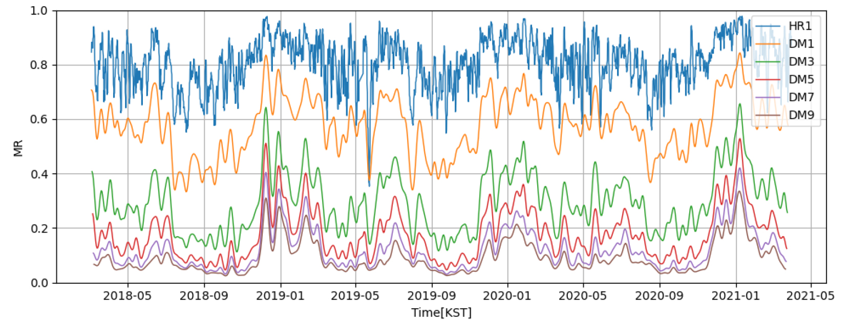
MR has seasonal trends where the missing is most excessive in winter between November and February and rarely in autumn between September and October.
Figs. 4 and 5 show the variation of the spatial distribution of missing data according to DMn and kernel size, as illustrated in Fig. 2c above, for the same date, March 25, 2018, respectively. The DMn method effectively reduced missing grids by 7.78% at DM9 while the kernel method was ineffective, having 44.09% at the eight-by-eight kernel size, since the individual missing grid was clustered with one another and the kernel size was not enough to obtain a valid grid. This result proves that spatial integration is not preferable to temporal integration in removing missing points.
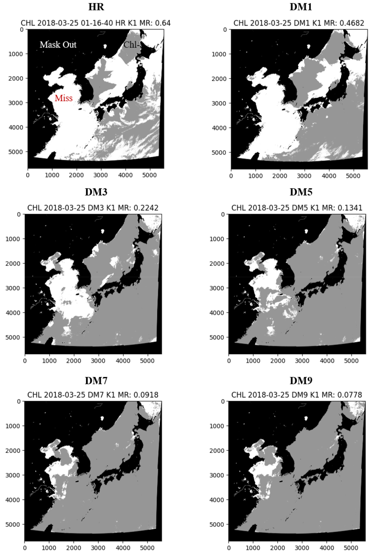
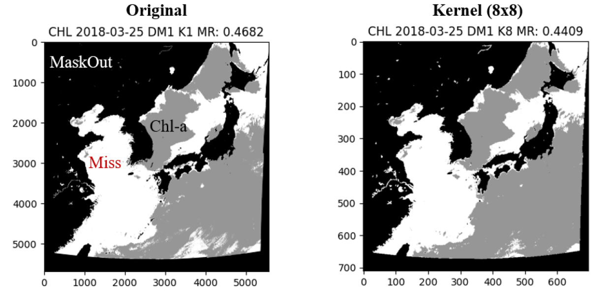
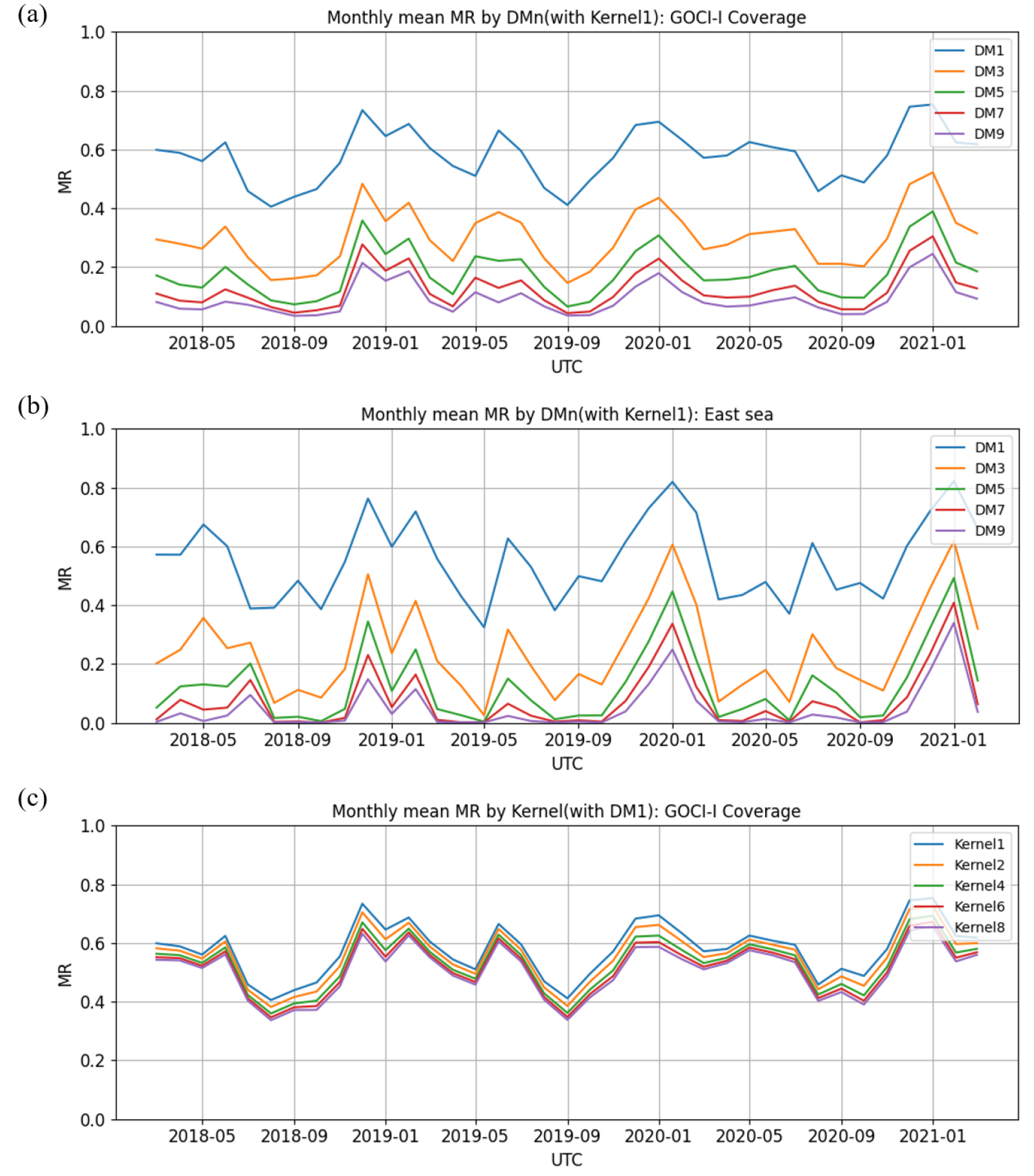
Fig. 6a and c shows the monthly mean variation of MR of temporal and spatial integration for GOCI-I coverage, respectively. DMn method shows more effectiveness than the kernel method in reducing missing points. The seasonality becomes more evident than the variation of DMn (Fig. 3). On the other hand, the monthly variation of MR i n the East sea is not significantly different from that of GOCI-I coverage in the overall trend (Fig. 6b).
The error of estimation in the missing grids is highly affected by the MR and the pattern of missing-grids spatial distribution. Therefore, a certain level of reducing MR is required to estimate within the allowable error range considering spatial correlation since the higher MR, the higher the estimation error. Hair Jr. et al. (2010) suggests that 10% or less missing is permissible. However, despite the of DMn increase up to nine, there was no perfect reach to 10% for the whole period (Fig. 3). Thus, it may consume more data for up to a month to meet the MR degrading temporal resolution.
Therefore, it is required to analyze the variation of estimation error according to the reduction of the MR since the reduction of estimation error is a fundamental criterion. In the practical aspect, around 20% MR is appropriate if the temporal resolution is maintained for around five days. The appropriate MR needs to be re-determined considering allowable errors or unavoidable estimation errors because stricter values may show differences depending on the estimated items other than chlorophyll in the missing grids.
This is the trade-off between the decrease in the temporal resolution and the decrease in MR. An optimization issue is balancing benefits and losses from the reduced analytic resolution. The 20% MR and the five-days temporal resolution are presented as the optimal reference conditions in this analysis. By introducing an appropriate cost function, this condition can be changed.
Variation of Moran’s I for different integrating periods
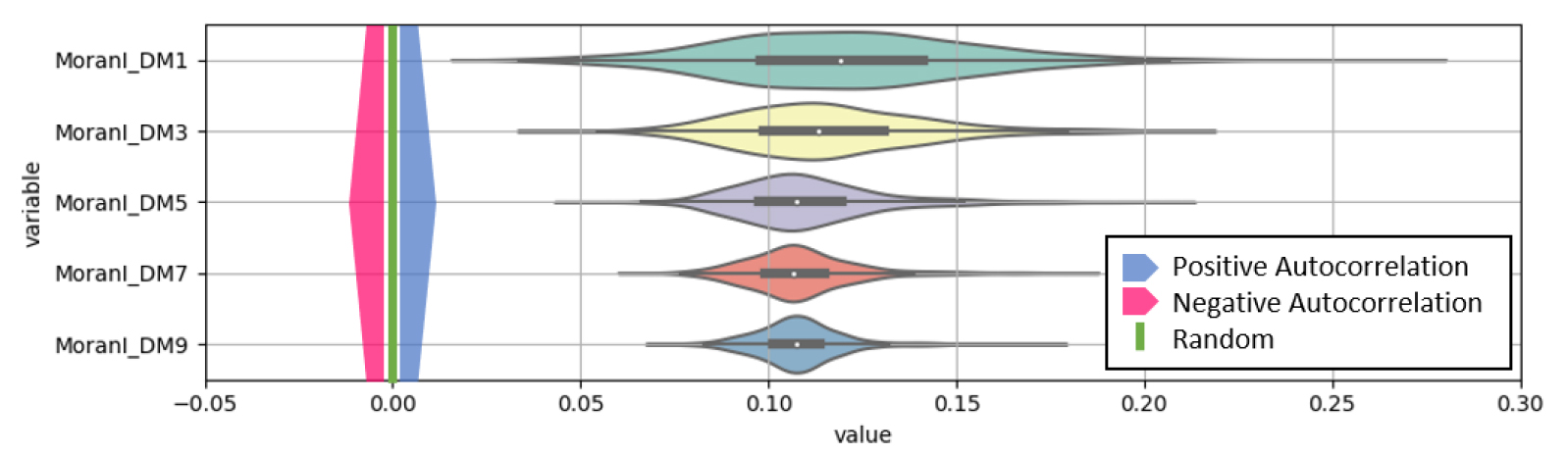
Moran’s I, one of the spatial autocorrelation indices, indicate that spatial points have autocorrelation when the value is farther from zero. In detail, values over zero indicate that spatial points have a positive autocorrelation where the attribute of points is clustered neighbor to neighbor. In contrast, under zero indicates the negative autocorrelation where the points attribute is opposite neighbor to neighbor like check pattern distribution. On the other hand, values closer to zero indicate that spatial points have a random distribution.
Daily Moran’s I was computed for March 4, 2018, to March 26, 2021, and the overall coverage of GOCI-I using 100-by-100 rescaled DMn (Fig. 7a). Overall DMn ranges from 0.03 to 0.26. DM1 shows the highest variation while DM9 shows the lowest variation. The Moran’s I values become lower with the increasing number of integrating periods and become stable due to lower variation.
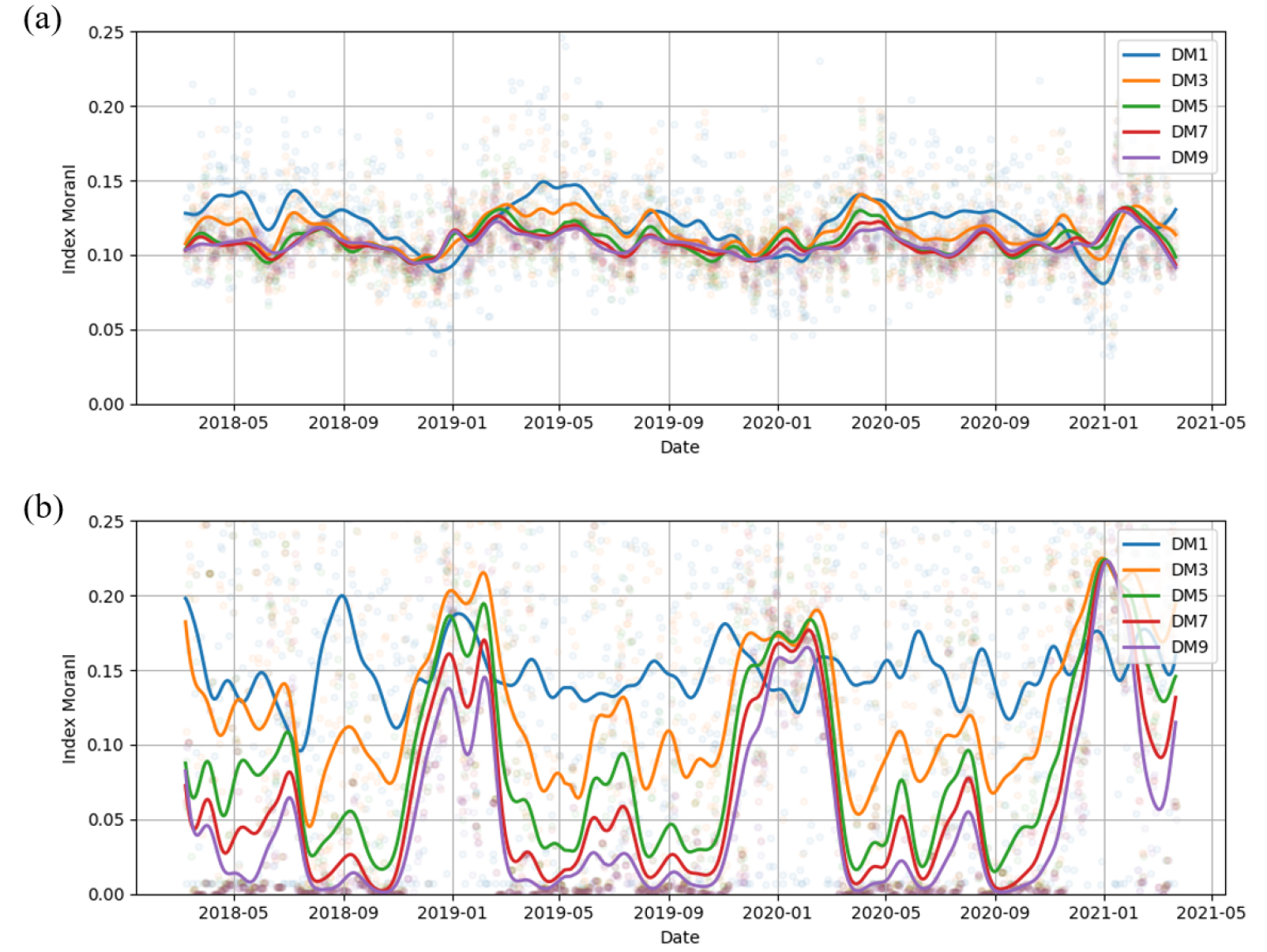
In addition, daily Moran’s I for the East sea was also computed (Fig. 7b). Overall DMn ranges from 0.00 to 0.36. From DM3, the seasonality of Moran’s I become apparent, showing the highest in winter and the lowest in autumn.
Distributions of Moran’s I for missing grids of daily DMn were compared using a violin plot that illustrates the distribution of data and quantile simultaneously (Fig. 8). The violin-shaped curved area represents the distribution of data. The black-flatten square in the violin indicates the inter-quantile range between 25%(Q1) and 75%(Q3). The white dot in the black square indicates the median value. A small decrease in median between DMn represents spatial autocorrelation is less affected by the temporal integration period. The reduced variance indicates that the spatial autocorrelation is gradually stable.
Variation of K-function for different integrating periods
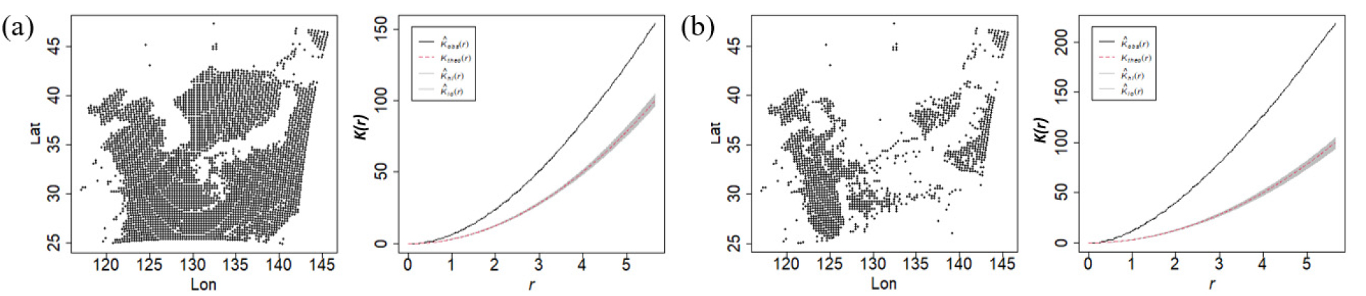
The comparison of K-function was made between DM1 and DM5 on March 21, 2018. As mentioned in section 2.4, the spatial point distribution analysis is based on the null hypothesis that the individual point in the region of interest is independent of others and has complete spatial randomness.
The observations K of DM1 values are greater than those of theoretic CSR values on every two points’ distance r when the missing prevails overall sea (Fig. 9). Thus the spatial distribution is determined as clustered and not in a random state. Likewise, DM5 also shows clustered distribution and none of the randomness.
Seasonality of MR
Periodical trends were found in every time-series plot (Figs. 3, 6 and 7). The Periodogram was used to detect superior frequency and period, representing seasonality. Three frequencies were detected through F-values and F-critical values.
F-test and Whittle-test were made for the three frequencies (Table 3). The seasonal periods, the value of inversed superior frequencies, were a year, half-year, and a quarter. Because every observed of the three periods was above the critical g-value of 0.016, the null hypothesis of none-seasonality is rejected, and they are considered as significant periods which are representative of seasonality.
4. Summary & Conclusions
This note described how missing grids are distributed in amount, spatial pattern, and seasonality aspects. We also answered three questions 1) what is the optimal choice to reduce the missing ratio 2) do the missing grids randomly distributed without pattern 3) Whether the missing ratio has seasonality and what is the interval.
The missing grids of GOCI-1 satellite images are caused by high aerosol ratio, atmospheric correction failure, clouds, and others. The average MR of GOCI-I chlorophyll product was approximate 80±15%. A comparison between temporal and spatial integration was made to reduce the MR. Consequently, temporal integration is revealed as a better method than spatial one. The five-days temporal integration reduced the number of missing data by 20% significantly while spatial integration was not practical where it reduced the missing data by 40 to 60%. The spatial distribution of missing grids was analyzed through Moran’s I, a spatial autocorrelation index, and Ripley K, a spatial distribution function. Both methods are based on the null hypothesis of complete spatial random (CSR). The test result shows that the null hypothesis is rejected and reveals that the missing pattern is not random but clustering weakly. The seasonality of MR and its significant period was confirmed through Fisher G-test. The result shows the MR has yearly, half-yearly, and quarter-yearly component exists. In the future study, we plan to generate the complete chlorophyll product where the missing at sea is filled, considering estimation error, with a week-level resolution and 250m or less spatial resolution using the GOCI-I product based on the result of this report.
