1. Introduction

The explosive growth in ocean data and model resolutions is rapidly outpacing the capabilities of traditional CPU computing (Vance et al. 2019; Delmas and Soulaïmani 2022; Beech et al. 2024). Many ocean models and data assimilation schemes still depend on CPUs, which are built with a small number of powerful and versatile cores (Ciżnicki et al. 2012; Zhang et al. 2012). Despite its usual effectiveness, this architecture becomes inefficient when faced with the massive and repetitive operations required for high-resolution ocean analyses (Häfner et al. 2021;Yuan et al. 2024; Porter and Heimbach 2025). However, GPUs contain thousands of smaller cores designed for parallel processing, enabling them to execute a large number of calculations simultaneously (Keckler et al. 2011; Navarro et al. 2014). This fundamental difference allows GPUs to deliver orders-of-magnitude accelerations over CPU-based approaches for ocean modeling (Bleichrodt et al. 2012; Xu et al. 2015; Zhao et al. 2017; Silvestri et al. 2025) and data assimilation (De Luca et al. 2021).

Although GPUs have been rapidly adopted in many scientific fields, their use in ocean modeling and assimilation remains limited. Major community ocean models such as MOM6 (Adcroft et al. 2019) and ROMS (Shchepetkin and McWilliams 2005) have not yet transitioned entirely to GPU architectures, and most implementations continue to rely on CPUs. Although experimental efforts and prototype tools have demonstrated the potential of GPU acceleration, the widely used data assimilation frameworks are still CPU-based and the operational data assimilation systems have not yet been coupled with GPUs (Martin et al. 2025). This slow transition is largely because of the extensive legacy of CPU-based Fortran codes, whose adaptation to the GPU architecture calls for an overhaul (Zhao et al. 2017; Vanderbauwhede and Davidson 2018; Porter and Heimbach 2025). Consequently, most operational ocean prediction systems are still implemented using CPUs, even as the scientific community increasingly demands higher-resolution products and near-real-time applications. Considering this, GPU acceleration is no longer optional but essential.

This study demonstrates the advantages of GPU computing through a classical yet computationally demanding example: Optimal Interpolation (OI). OI has long been used in oceanography because of its analytical rigor, cost-effectiveness, and relatively straightforward implementation. Additionally, global-scale applications involve nontrivial computational demands, rendering OI a suitable example for testing GPU acceleration. Furthermore, OI shares mathematical formulations with widely used data assimilation schemes such as the Ensemble Kalman Filter (Evensen 1994) and Ensemble Optimal Interpolation (Evensen 2003) in operational ocean prediction systems (Chang et al. 2024; Jin et al. 2024), which provide strong scalability for broader applications. The OI was implemented on a modern GPU platform to evaluate the efficiency gains while maintaining methodological fidelity. As a practical test case, GPU-accelerated OI was applied to reconstruct the global ocean surface partial pressure of CO₂ (pCO₂), which is a key variable for quantifying air-sea CO₂ fluxes and assessing the role in the global carbon cycle (Iida et al. 2015; Roobaert et al. 2024). Although existing global pCO₂ products provide useful large-scale features, they still contain uncertainties associated with sparse observations and methodological assumptions. Data assimilation of pCO₂ observations therefore plays a critical role in reducing these uncertainties. This demonstration highlights the computational benefits of GPU-based assimilation and its potential to support timely and higher-resolution ocean prediction systems.

The remainder of this paper is organized as follows. Section 2 describes the datasets, principles of OI, and its GPU-based implementation. Section 3 presents the reconstructed global ocean surface pCO₂ fields. Section 4 benchmarks the computational performance of the GPU and CPU implementations, highlighting efficiency gains. Finally, Section 5 summarizes the findings and provides concluding remarks.

2. Data and Method

Data sources

The analysis focuses on the global ocean surface, using the background field of pCO₂ from SeaFlux v2021.04 (https://doi.org/10.5281/zenodo.5482547), which provides 1° global monthly pCO₂ estimates between 1990–2019 (Fay et al. 2021). This product was developed within the framework of the Surface Ocean pCO₂ Mapping Intercomparison (SOCOM) project (Rödenbeck et al. 2015), an international effort that systematically compared and combined multiple mapping approaches. The spco2_filler field from SeaFlux, based on adjusted climatology (Landschützer et al. 2020), was used within this framework to provide a spatially complete and consistent background for the OI assimilation experiments. The spatial distribution of the long-term mean pCO₂ from SeaFlux is shown in Fig. 1a.

Fig. 1.

Spatial distribution of (a) annual mean ocean surface pCO₂ from background (μatm) and (b) time-accumulated number of observations, and (c) monthly time-series of the number of global bin-averaged observations

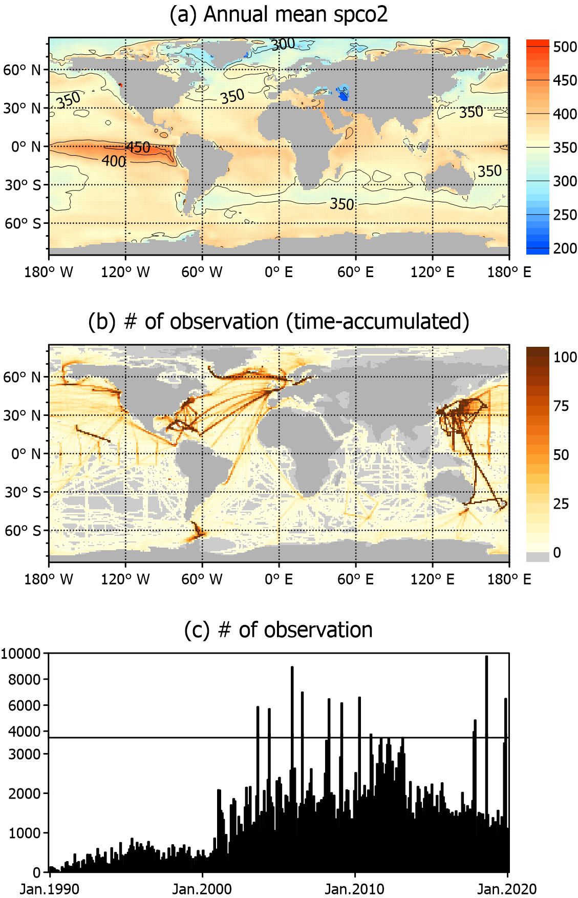
To constrain data assimilation, three major observational compilations were used: the Surface Ocean CO₂ Atlas (SOCAT), the Lamont-Doherty Earth Observatory (LDEO) database, and underway observations from Korea Institute of Ocean Science & Technology (KIOST). SOCAT provides the most comprehensive global collection of surface ocean CO₂ data (Bakker et al. 2016) and contains more than 41 million quality-controlled observations from 1957 to 2023 (https://socat.info). It primarily includes underway shipboard measurements and data from fixed time-series stations that offer both wide spatial coverage and long-term reference points. As SOCAT provides the fugacity of CO₂ (fCO₂) rather than pCO₂, fCO₂ was converted to pCO₂ using the f2pco2 function in the seacarb R package (https://doi.org/10.32614/CRAN.package.seacarb). The LDEO V2019 database (https://www.ncei.noaa.gov/data/oceans/ncei/ocads/metadata/0160492.html) was one of the earliest global efforts to curate surface water pCO₂ records. Although most of its content overlaps with that of SOCAT, it includes a unique time-series and carefully calibrated cruise data. Underway pCO₂ measurements collected by KIOST research vessels between 2003 and 2019 were also included, which spanned the East/Japan Sea, the East China Sea, and a limited number of cruises in the North Pacific. These data complement global compilations and provide valuable constraints for regions in which international datasets are sparse.

For assimilation, all the observations were aggregated monthly and bin-averaged onto a 0.25° grid, and all the available measurements in each bin were combined into monthly means (Fig. 1b). These binned observations were assimilated into a 1° background field, and thus the resulting analysis fields are also produced at 1° resolution. The spatial distribution shows particularly dense coverage in the North Pacific and North Atlantic, whereas open ocean regions such as the South Pacific, South Atlantic, and South Indian Ocean are poorly observed. To match the background period (1990–2019), the observational dataset was restricted to the same time range. The global time-series of bin-averaged observations demonstrated a sharp increase in data availability after 2000, with an average of 1,193 bins containing observations per month and a maximum of 9,770 in the most densely sampled months (Fig. 1c).

Optimal Interpolation

The OI method combines the background with observations to generate an improved analysis field. The fundamental formulae are as follows:

where X^a and X^b denote the state vectors of the analysis and background fields, respectively. Y indicates the observation state vector and operator H projects the background field into the observation points. Gain matrix W is defined as follows:

where B and R denote the background and observational error covariance matrices, respectively. The superscript T denotes the transpose, and -1 denotes the matrix inverse.

Background error covariance B was prescribed using a Gaussian correlation function with an e-folding length scale of 250 km. This value is broadly consistent with the previous estimates of the spatial decorrelation scale of the ocean surface fCO₂ variability (~400 ± 250 km; Jones et al. 2012), however, it was set slightly shorter to better capture the local variability in the complex Korean marginal seas, where dense observations are available (Fig. 1b). The background error variance at each grid point (diagonals of B) and the observational error variance (diagonals of R) were both set to 10 (μatm)². Although this is arbitrary, it was chosen to balance the background and observational influences in the absence of additional quality control. It is the relative magnitudes of B and R, rather than their absolute values, that determines the OI analysis. This indicates that the specific choice of 10 (μatm)² is not important in itself. The observations were assumed to be independent, i.e., R is diagonal.

The full background error covariance matrix B of size n_s × n_s, where n_s is the number of background grid points, was not explicitly constructed because this would be computationally prohibitive. Instead, only the covariance terms required for the OI analysis were directly computed, namely BH^T (n_s × n_o) and HBH^T (n_o × n_o), where n_o is the number of observation points. Both represent background error covariances: BH^T between the background and observation points and HBH^T among the observation points.

OI implementation for GPU

A grid-chunking strategy was employed to accelerate the OI computation. The global background grid (n_s) was divided into smaller chunks of size n_c and OI updates were performed independently for each chunk (Fig. 2a). The OI analysis for chunk c can be written as:

where subscript c denotes the chunk. Matrix (HBH^T + R)^-1 and vector (Y – HX^b) have dimensions of n_o × n_o and n_o × 1, respectively; therefore their product (HBH^T + R)^-1(Y – HX^b) is manageable and can be computed once for use in all the chunks (Fig. 2a). Each chunk requires only the calculation of (BH^T)_c with a size of n_c × n_o. In this study, chunks were not defined based on geographic regions but were sequentially divided for computational convenience, since the chunking strategy does not affect the OI results.

Fig. 2.

Schematics of (a) chunk-based and (b) chunk-based sequential Optimal Interpolation (OI). The state vector of length n_s is partitioned into chunks of size n_c, and the observations (n_o) are grouped into batches of size n_b for sequential OI

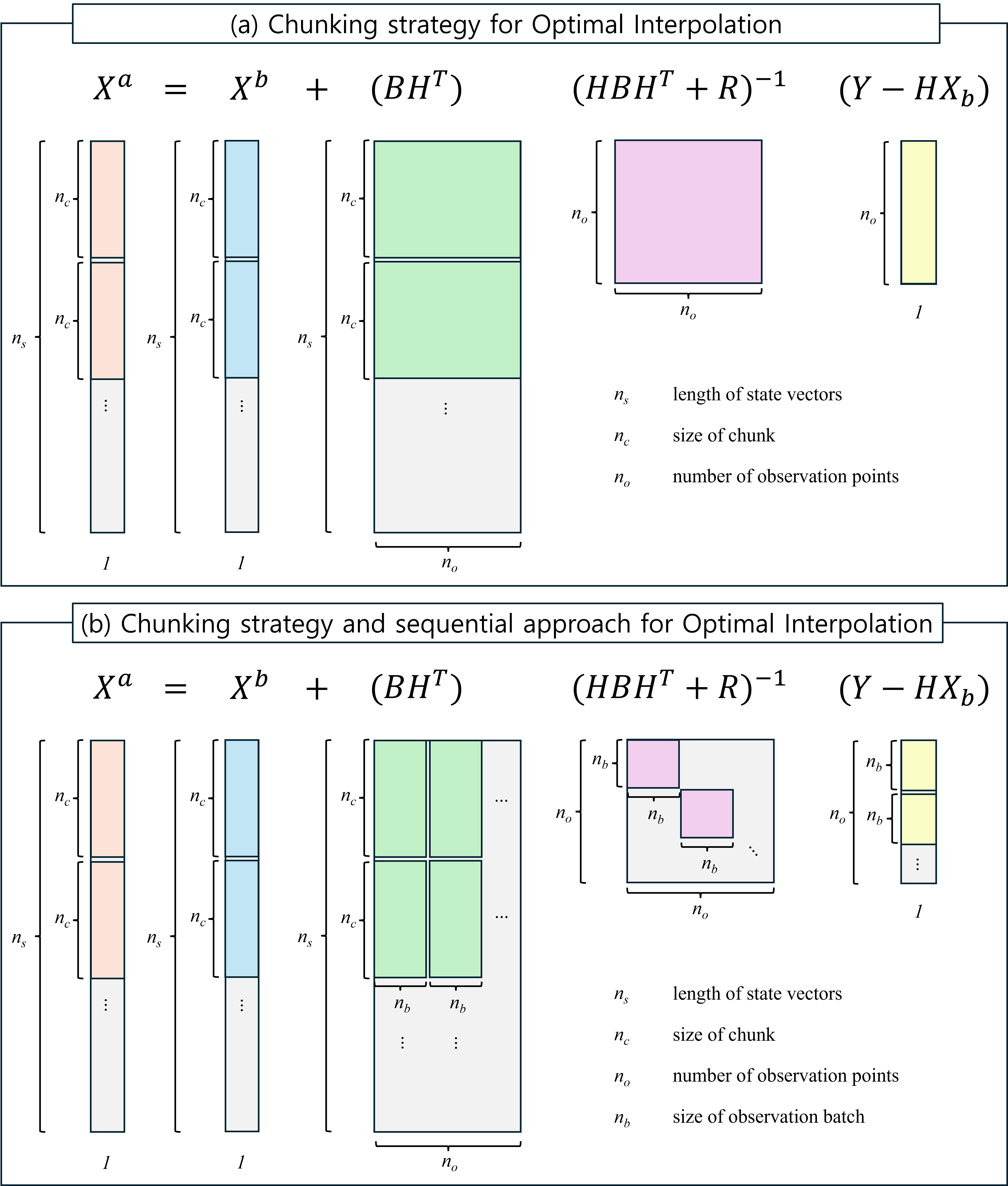
Although the chunk-based strategy facilitates efficient implementation, its memory demand is still huge, because the term (HBH^T + R)^-1 scales as n_o² (Fig. 2a). In an operational ocean prediction system, the number of practical observation points in the 3-dimensional field at one step of data assimilation can reach the order of 10⁵. This would require approximately 80 GB of memory, which is already beyond the capacity of modern GPUs with 32GB of VRAM. To overcome this limitation, a sequential approach (Houtekamer and Mitchell 2001) was applied in which the full observation set (n_o) was divided into smaller batches of size n_b (Fig. 2b). Here, a chunk refers to a subset of background grid points, whereas a batch denotes a subset of observations. Instead of applying the entire observation set to a single update, the sequential method assimilates each batch sequentially and updates the analysis field iteratively. This reduces memory usage by limiting the matrix operations to n_b × n_b size. However, this approach can cause small discrepancies relative to the all-at-once observation updates. In the present experiments, fewer than 10,000 observations were used per update; therefore, the all-at-once method is feasible. However, sequential OI is also considered, with future operational applications in mind, where more than 10⁵ observations may need to be assimilated.

The chunk-based sequential OI implementation was further accelerated using GPU parallelization with the CuPy library in Python (https://cupy.dev). Many Python users rely on NumPy for array operations (Harris et al. 2020), and CuPy provides a NumPy-compatible interface that enables most matrix operations in the OI update to be executed on CUDA-enabled GPUs with minimal modifications. In the GPU runs, both the grid chunk and observation batch loops were executed sequentially and the matrix operations inside each loop were performed in parallel on the GPU. Although data reading and storage were handled by the CPU, nearly all the subsequent computations were performed on the GPU. This design substantially reduced the runtime compared with the CPU-only experiments (see Section 4.1). The chunk-based OI algorithm was also executed on CPUs using NumPy, both in the single-core mode and in parallel with 8-core and 24-core configurations, to provide baselines for performance comparison. In single-core mode, the grid chunk loop was executed sequentially, and in multi-core mode, it was split across the CPU cores and executed simultaneously.

3. Test Case: Global pCO₂ Analysis

The OI update is illustrated for February 2013 (Fig. 3a–d), as a representative snapshot to show the spatial characteristics of the analysis fields. The background field (Fig. 3a) provides a gap-free global coverage with elevated pCO₂ (> 450 μatm) in the eastern equatorial Pacific and coastal regions in the Northern Hemisphere, contrasted by relatively low pCO₂ (< 350 μatm) across midlatitude Northern Hemisphere and high-latitude Southern Hemisphere. The spatial distribution was not significantly different from that of the long-term average field (Fig. 1a). The observations comprised numerous underway tracks, particularly across the North Pacific, North Atlantic, and Southern Ocean, along with several fixed-point stations worldwide (Fig. 3b). Although the OI analysis (Fig. 3c) closely resembled the background, the increments (analysis minus background; Fig. 3d) revealed local adjustments near the observations. The magnitude of the update remained moderate, indicating that the OI nudges the background toward observations without introducing noticeable artifacts. The resulting analysis is available at https://doi.org/10.22711/idr/1105.

A comparison of the time-series of the area-averaged pCO₂ shows that the analysis closely follows the background at the global scale (Fig. 3e), with larger departures in the Northwest Pacific, where observations were denser (Fig. 3f). These results confirm that OI behaves as expected, with sharper local corrections in observation-rich regions, whereas observation-poor regions retain background characteristics. Overall, the resulting pCO₂ analysis fields remain broadly consistent with the SeaFlux background, while local pCO₂ features reflect observational information more explicitly. In particular, the inclusion of observations around Korea is expected to improve the representation of regional air-sea CO₂ exchange, which may be beneficial for quantifying carbon fluxes in this region. This test case primarily focuses on computational performance and methodological consistency, without aiming for a detailed validation of the pCO₂ analysis fields.

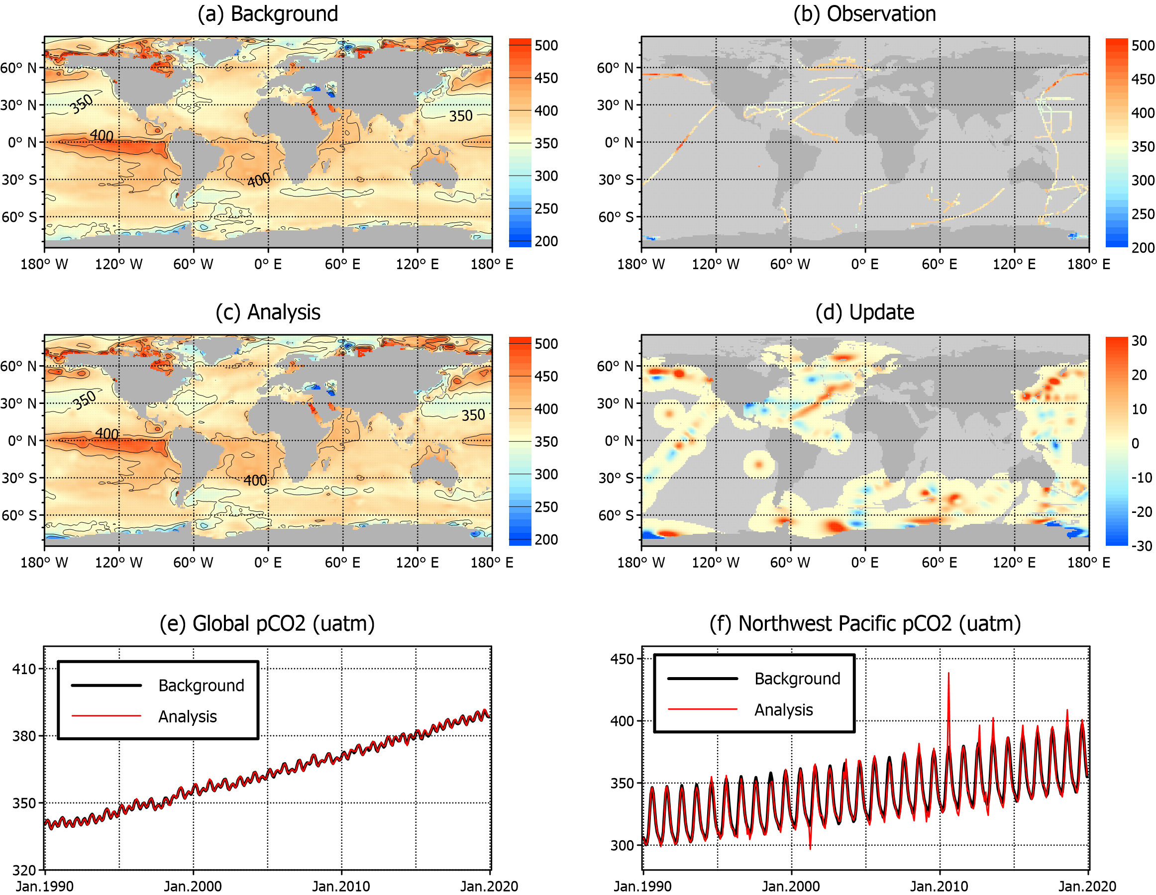
Fig. 3.

(a–d) Spatial distribution of (a) background, (b) observations, (c) OI analysis, and (d) update (analysis minus background) of ocean surface pCO₂ (μatm) in February 2013. (e–f) Time-series of area-averaged pCO₂ from the background (thick black line) and analysis (red line) fields in the (e) global and (f) Northwest Pacific (125–145°E, 25–45°N)

4. Performance Benchmarking

GPU vs CPU

Benchmarking experiments were performed on a workstation with an NVIDIA RTX 5090 GPU (32 GB of GDDR6 VRAM), Intel Xeon W7-3465X CPU (28 cores, 3.2 GHz clock), 256 GB system memory, and WD Black 850x NVMe SSD (8 TB). Comparisons were performed using chunk sizes ranging from 1,000 to 50,000 under an all-at-once observation update, where the maximum number of observations per step was slightly less than 10,000. The OI background field for pCO₂ comprised 44,598 grid points. Therefore, a chunk size of 50,000 effectively and simultaneously used the entire background grid. CPU runs were executed in single-core and multi-core modes (i.e., 1X, 8X, and 24X). Each test was repeated five times, and the average runtime was calculated after discarding the fastest and slowest runs. The input/output operations, which required approximately 6 s per run, were included in the runtime. The experiment names follow the format of Processor-Chunk size, for example, GPU-01k for a GPU run with a chunk size of 1,000 and CPU-24X-50k for a 24-core CPU run with a chunk size of 50,000. The speedup ratio is defined as the runtime of the baseline (CPU-1X-01k; Table 1) divided by that of each test case, with values greater (less) than one indicating acceleration (slowdown).

The benchmarking results clearly highlight the advantages of GPU acceleration. GPU runs such as GPU-50k were up to 35 times faster than that of the single-core CPU baseline (CPU-1X-01k) and approximately 12 times faster than that of the multi-core CPU runs (CPU-8X-01k). The runtime on GPUs decreased with larger chunk sizes, and converged beyond 5,000 grid points, indicating that GPU efficiency was saturated once sufficiently large chunks were used.

However, the CPU performance exhibited a different pattern. Although the efficiency gains diminished between 8 and 24 cores, multi-core settings reduced the runtime compared with the single-core case (1,338 s for CPU-1X-01k, 521 s for CPU-8X-01k, and 457 s for CPU-24X-01k). The CPU runtime generally increased with larger chunk sizes; for example, it increased from 1,338 s at 1,000 points to 1,732 s at 50,000 points in the single-core case. This slowdown presumably reflects the memory bandwidth limitations when larger chunks exceed cache capacity (Patterson and Hennessy 2016), a behavior also observed in multi-core runs. Because the full domain contained 44,598 grid points, the CPU experiments with chunk sizes above 5,000 (for 8 cores) or 2,000 (for 24 cores) no longer balanced the workload effectively across cores. Consequently, for the chunk sizes of 10k, 20k, and 50k, the runtimes of the 8X and 24X parallel modes were nearly identical (Table 1). Notably, although the multi-core 50k cases should have been equivalent to a single-core computation (CPU-1X-50k; 1,732 s), CPU-8X-50k (1,485 s) and CPU-24X-50k (1,486 s) achieved slightly better performances. This modest improvement likely comes from the fact that Python relies on an optimized linear algebra library (OpenBLAS) for matrix operations, which can automatically use multiple CPU cores during the matrix operations outside the chunk loops. In contrast, in the single-core mode, these processes are handled solely by a single core.

Sequential OI tests with GPU

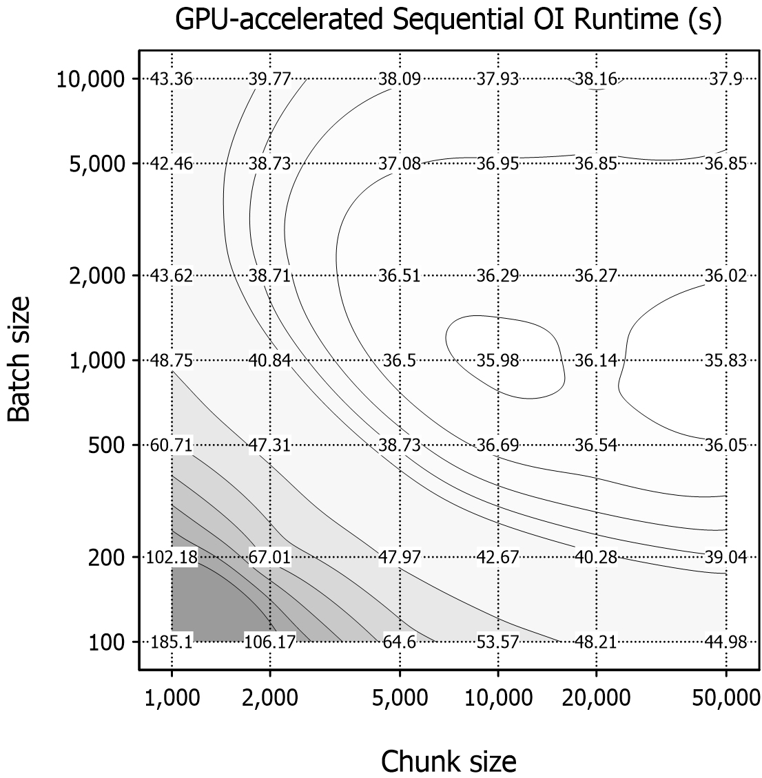
Sequential OI sensitivity tests were only performed on the GPU by varying both the chunk size (1,000–50,000) and batch size (100–10,000) to evaluate the runtime performance (Fig. 4). Typically, the runtime decreased as the batch size increased because smaller batches used less memory per operation and required more repetitions, which slowed the performance. Larger batches reduced repetition and improved efficiency; however, the benefit became negligible beyond the batch size of approximately 2,000. The fastest runtimes were consistent within the range n_b = 1,000–2,000, whereas the performance declined at larger n_b values (e.g., 5,000 or 10,000). This decline likely reflects the increasing computational cost of the larger matrix inversion (HBH^T + R)^-1. Chunk size also has a strong effect on performance. Larger chunks reduced loop iterations and accelerated computations, whereas smaller chunks increased the repetition overhead and slowed the runtimes. The fastest runtime was obtained at the maximum chunk size (50,000) with a batch size of 1,000. These results indicate that although larger chunk sizes are consistently beneficial, batch sizes have an optimal range of approximately 1,000–2,000 rather than improving monotonically with size.

Fig. 4.

Runtimes of GPU-accelerated sequential OI as a function of chunk size (1,000–50,000) and batch size (100–10,000)

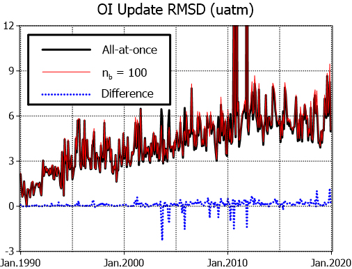
Beyond runtime, the consistency of sequential OI with the all-at-once approach (n_b = 10,000) was also evaluated. The spatial root-mean-square difference (RMSD) time-series was calculated between the background and analysis fields from the all-at-once (n_b = 10,000) run and the sequential OI with n_b = 100 (Fig. 5). The all-at-once update typically modified the background by approximately 3–6 µatm at the global scale. When sequential OI with n_b = 100 was applied, the resulting analysis fields exhibited similar temporal variations, with only minor deviations from the all-at-once case. Since the n_b = 100 case represents the smallest batch size considered and thus represents the worst-case scenario, the consistency observed for this case implies even smaller RMSD differences for larger batch sizes (not shown). This finding indicates that sequential OI introduce only minor discrepancies, as reported by Houtekamer and Mitchell (2001). Although it requires slightly longer runtimes (~45 s) than the all-at-once case (~38 s), sequential OI provides a practical strategy when memory limitations prevent all-at-once implementation. In addition, the sequential approach can be computationally advantageous under optimal conditions (e.g., n_b = 1,000), achieving slightly shorter runtimes than the all-at-once case.

Fig. 5.

Time-series of RMSD between the background and the analysis from all-at-once observation update (thick black line) and from sequential OI with a batch size of 100 (red line) overlaid with their difference (blue dotted line)

5. Summary and Concluding Remarks

This study highlights the benefits of GPU acceleration for the OI of global ocean surface pCO₂. A chunk-based sequential OI scheme was implemented using 30 years of monthly background field and bin-averaged observations. A test case for February 2013 confirmed that the OI system successfully assimilated observation data into the background. Performance benchmarking demonstrated substantial acceleration with the GPU implementation, achieving runtimes up to 35 times faster than that of a single-core CPU baseline and approximately 12 times faster than that of multi-core CPU runs. The GPU performance was improved by increasing the chunk size, with only modest gains beyond 5,000. Sensitivity tests further showed that batch sizes of 1,000–2,000 provided the best runtimes. Sequential OI produced analysis fields that were nearly identical to those from the all-at-once update, with a moderate runtime penalty.

This study provides a practical pathway for applying GPUs in data assimilation. As an initial step toward GPU-based ocean data assimilation, a relatively simple test case with OI to 1° global pCO₂ fields to examine the feasibility of GPU acceleration. The proposed OI schemes are compatible with operational ocean prediction systems based on Ensemble Optimal Interpolation (Jin et al. 2024). The operational system must assimilate large observations into high-resolution three-dimensional model grids, which imposes prohibitive demands on memory and computational power. An efficient GPU implementation can satisfy these computational requirements, whereas a chunk-based sequential OI algorithm alleviates the memory burden. The GPU-based system also achieved more than an order-of-magnitude speedup over the fastest CPU configuration in this study, and such a clear advantage of GPUs is expected to remain even when using other recent CPU and GPU hardware. This transition to GPU-based data assimilation is expected to reduce the prediction time. Moreover, if numerical ocean models are migrated to GPU platforms, an even faster and more efficient ocean prediction system can be realized.